The graph_tool module provides a Graph class and several algorithms that operate on it. The internals of this class, and of most algorithms, are written in C++ for performance, using the Boost Graph Library.
The module must be of course imported before it can be used. The package is subdivided into several sub-modules. To import everything from all of them, one can do:
>>> from graph_tool.all import *
In the following, it will always be assumed that the previous line was run.
An empty graph can be created by instantiating a Graph class:
>>> g = Graph()
By default, newly created graphs are always directed. To construct undirected graphs, one must pass a value to the directed parameter:
>>> ug = Graph(directed=False)
A graph can always be switched on-the-fly from directed to undirected (and vice versa), with the set_directed() method. The “directedness” of the graph can be queried with the is_directed() method,
>>> ug = Graph()
>>> ug.set_directed(False)
>>> assert(ug.is_directed() == False)
A graph can also be created by providing another graph, in which case the entire graph (and its internal property maps, see Property maps) is copied:
>>> g1 = Graph()
>>> # ... construct g1 ...
>>> g2 = Graph(g1)                 # g1 and g2 are copies
Above, g2 is a “deep” copy of g1, i.e. any modification of g2 will not affect g1.
Once a graph is created, it can be populated with vertices and edges. A vertex can be added with the add_vertex() method, which returns an instance of a Vertex class, also called a vertex descriptor. For instance, the following code creates two vertices, and returns vertex descriptors stored in the variables v1 and v2.
>>> v1 = g.add_vertex()
>>> v2 = g.add_vertex()
Edges can be added in an analogous manner, by calling the add_edge() method, which returns an edge descriptor (an instance of the Edge class):
>>> e = g.add_edge(v1, v2)
The above code creates a directed edge from v1 to v2. We can visualize the graph we created so far with the graph_draw() function.
>>> graph_draw(g, vertex_text=g.vertex_index, vertex_font_size=18,
...            output_size=(200, 200), output="two-nodes.pdf")
<...>
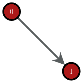
A simple directed graph with two vertices and one edge, created by the commands above.
With vertex and edge descriptors, one can examine and manipulate the graph in an arbitrary manner. For instance, in order to obtain the out-degree of a vertex, we can simply call the out_degree() method:
>>> print(v1.out_degree())
1
Analogously, we could have used the in_degree() method to query the in-degree.
Note
For undirected graphs, the “out-degree” is synonym for degree, and in this case the in-degree of a vertex is always zero.
Edge descriptors have two useful methods, source() and target(), which return the source and target vertex of an edge, respectively.
>>> print(e.source(), e.target())
0 1
The add_vertex() method also accepts an optional parameter which specifies the number of vertices to create. If this value is greater than 1, it returns an iterator on the added vertex descriptors:
>>> vlist = g.add_vertex(10)
>>> print(len(list(vlist)))
10
Edges and vertices can also be removed at any time with the remove_vertex() and remove_edge() methods,
>>> g.remove_edge(e)                               # e no longer exists
>>> g.remove_vertex(v2)                # the second vertex is also gone
Note
Removing a vertex is an \(O(N)\) operation. The vertices are internally stored in a STL vector, so removing an element somewhere in the middle of the list requires the shifting of the rest of the list. Thus, fast \(O(1)\) removals are only possible if one can guarantee that only vertices in the end of the list are removed (the ones last added to the graph).
Removing an edge is an \(O(k_{s} + k_{t})\) operation, where \(k_{s}\) is the out-degree of the source vertex, and \(k_{t}\) is the in-degree of the target vertex.
Each vertex in a graph has an unique index, which is numbered from 0 to N-1, where N is the number of vertices. This index can be obtained by using the vertex_index attribute of the graph (which is a property map, see Property maps), or by converting the vertex descriptor to an int.
>>> v = g.add_vertex()
>>> print(g.vertex_index[v])
11
>>> print(int(v))
11
Note
Removing a vertex will cause the index of any vertex with a larger index to be changed, so that the indexes always conform to the \([0, N-1]\) range. However, property map values (see Property maps) are unaffected.
Since vertices are uniquely identifiable by their indexes, there is no need to keep the vertex descriptor lying around to access them at a later point. If we know its index, one can obtain the descriptor of a vertex with a given index using the vertex() method,
>>> v = g.vertex(8)
which takes an index, and returns a vertex descriptor. Edges cannot be directly obtained by its index, but if the source and target vertices of a given edge is known, it can be obtained with the edge() method
>>> g.add_edge(g.vertex(2), g.vertex(3))
<...>
>>> e = g.edge(2, 3)
Another way to obtain edge or vertex descriptors is to iterate through them, as described in section Iterating over vertices and edges. This is in fact the most useful way of obtaining vertex and edge descriptors.
Like vertices, edges also have unique indexes, which are given by the edge_index property:
>>> e = g.add_edge(g.vertex(0), g.vertex(1))
>>> print(g.edge_index[e])
1
Differently from vertices, edge indexes do not necessarily conform to any specific range. If no edges are ever removed, the indexes will be in the range \([0, E-1]\), where \(E\) is the number of edges, and edges added earlier have lower indexes. However if an edge is removed, its index will be “vacant”, and the remaining indexes will be left unmodified, and thus will not lie in the range \([0, E-1]\). If a new edge is added, it will reuse old indexes, in an increasing order.
Algorithms must often iterate through vertices, edges, out-edges of a vertex, etc. The Graph and Vertex classes provide different types of iterators for doing so. The iterators always point to edge or vertex descriptors.
In order to iterate through all the vertices or edges of a graph, the vertices() and edges() methods should be used:
for v in g.vertices():
    print(v)
for e in e.edges():
    print(e)
The code above will print the vertices and edges of the graph in the order they are found.
The out- and in-edges of a vertex, as well as the out- and in-neighbours can be iterated through with the out_edges(), in_edges(), out_neighbours() and in_neighbours() methods, respectively.
from itertools import izip
for v in g.vertices():
   for e in v.out_edges():
       print(e)
   for w in v.out_neighbours():
       print(w)

   # the edge and neighbours order always match
   for e,w in izip(v.out_edges(), v.out_neighbours()):
       assert(e.target() == w)
The code above will print the out-edges and out-neighbours of all vertices in the graph.
Note
The ordering of the vertices and edges visited by the iterators is always the same as the order in which they were added to the graph (with the exception of the iterator returned by edges()). Usually, algorithms do not care about this order, but if it is ever needed, this inherent ordering can be relied upon.
Warning
You should never remove vertex or edge descriptors when iterating over them, since this invalidates the iterators. If you plan to remove vertices or edges during iteration, you must first store them somewhere (such as in a list) and remove them only after no iterator is being used. Removal during iteration will cause bad things to happen.
Property maps are a way of associating additional information to the vertices, edges or to the graph itself. There are thus three types of property maps: vertex, edge and graph. All of them are handled by the same class, PropertyMap. Each created property map has an associated value type, which must be chosen from the predefined set:
| Type name | Alias |
|---|---|
| bool | uint8_t |
| int16_t | short |
| int32_t | int |
| int64_t | long, long long |
| double | float |
| long double | |
| string | |
| vector<bool> | vector<uint8_t> |
| vector<int16_t> | vector<short> |
| vector<int32_t> | vector<int> |
| vector<int64_t> | vector<long>, vector<long long> |
| vector<double> | vector<float> |
| vector<long double> | |
| vector<string> | |
| python::object | object |
New property maps can be created for a given graph by calling the new_vertex_property(), new_edge_property(), or new_graph_property(), for each map type. The values are then accessed by vertex or edge descriptors, or the graph itself, as such:
from itertools import izip
from numpy.random import randint

g = Graph()
g.add_vertex(100)
# insert some random links
for s,t in izip(randint(0, 100, 100), randint(0, 100, 100)):
    g.add_edge(g.vertex(s), g.vertex(t))

vprop_double = g.new_vertex_property("double")            # Double-precision floating point
vprop_double[g.vertex(10)] = 3.1416

vprop_vint = g.new_vertex_property("vector<int>")         # Vector of ints
vprop_vint[g.vertex(40)] = [1, 3, 42, 54]

eprop_dict = g.new_edge_property("object")                # Arbitrary python object. In this case, a dictionary.
eprop_dict[g.edges().next()] = {"foo": "bar", "gnu": 42}

gprop_bool = g.new_edge_property("bool")                  # Boolean
gprop_bool[g] = True
Property maps with scalar value types can also be accessed as a numpy.ndarray, with the get_array() method, or the a attribute, i.e.,
from numpy.random import random

# this assigns random values to the vertex properties
vprop_double.get_array()[:] = random(g.num_vertices())

# or more conveniently (this is equivalent to the above)
vprop_double.a = random(g.num_vertices())
Any created property map can be made “internal” to the corresponding graph. This means that it will be copied and saved to a file together with the graph. Properties are internalized by including them in the graph’s dictionary-like attributes vertex_properties, edge_properties or graph_properties (or their aliases, vp, ep or gp, respectively). When inserted in the graph, the property maps must have an unique name (between those of the same type):
>>> eprop = g.new_edge_property("string")
>>> g.edge_properties["some name"] = eprop
>>> g.list_properties()
some name      (edge)    (type: string)
Internal graph property maps behave slightly differently. Instead of returning the property map object, the value itself is returned from the dictionaries:
>>> gprop = g.new_graph_property("int")
>>> g.graph_properties["foo"] = gprop   # this sets the actual property map
>>> g.graph_properties["foo"] = 42      # this sets its value
>>> print(g.graph_properties["foo"])
42
>>> del g.graph_properties["foo"]       # the property map entry is deleted from the dictionary
Graphs can be saved and loaded in three formats: graphml, dot and gml. Graphml is the default and preferred format, since it is by far the most complete. The dot and gml formats are fully supported, but since they contain no precise type information, all properties are read as strings (or also as double, in the case of gml), and must be converted by hand. Therefore you should always use graphml, since it performs an exact bit-for-bit representation of all supported Property maps, except when interfacing with other software, or existing data, which uses dot or gml.
A graph can be saved or loaded to a file with the save and load methods, which take either a file name or a file-like object. A graph can also be loaded from disc with the load_graph() function, as such:
g = Graph()
#  ... fill the graph ...
g.save("my_graph.xml.gz")
g2 = load_graph("my_graph.xml.gz")
# g and g2 should be copies of each other
Graph classes can also be pickled with the pickle module.
A Price network is the first known model of a “scale-free” graph, invented in 1976 by de Solla Price. It is defined dynamically, where at each time step a new vertex is added to the graph, and connected to an old vertex, with probability proportional to its in-degree. The following program implements this construction using graph-tool.
Note
Note that it would be much faster just to use the price_network() function, which is implemented in C++, as opposed to the script below which is in pure python. The code below is merely a demonstration on how to use the library.
1 2 3 4 5 6 7 8 9 10 11 12 13 14 15 16 17 18 19 20 21 22 23 24 25 26 27 28 29 30 31 32 33 34 35 36 37 38 39 40 41 42 43 44 45 46 47 48 49 50 51 52 53 54 55 56 57 58 59 60 61 62 63 64 65 66 67 68 69 70 71 72 73 74 75 76 77 78 79 80 81 82 83 84 85 86 87 88 89 90 91 92 93 94 95 96 97 98 99 100 101 | #! /usr/bin/env python
# We probably will need some things from several places
import sys, os
from pylab import * # for plotting
from numpy.random import * # for random sampling
seed(42)
# We need to import the graph_tool module itself
from graph_tool.all import *
# let's construct a Price network (the one that existed before Barabasi). It is
# a directed network, with preferential attachment. The algorithm below is
# very naive, and a bit slow, but quite simple.
# We start with an empty, directed graph
g = Graph()
# We want also to keep the age information for each vertex and edge. For that
# let's create some property maps
v_age = g.new_vertex_property("int")
e_age = g.new_edge_property("int")
# The final size of the network
N = 100000
# We have to start with one vertex
v = g.add_vertex()
v_age[v] = 0
# we will keep a list of the vertices. The number of times a vertex is in this
# list will give the probability of it being selected.
vlist = [v]
# let's now add the new edges and vertices
for i in range(1, N):
# create our new vertex
v = g.add_vertex()
v_age[v] = i
# we need to sample a new vertex to be the target, based on its in-degree +
# 1. For that, we simply randomly sample it from vlist.
i = randint(0, len(vlist))
target = vlist[i]
# add edge
e = g.add_edge(v, target)
e_age[e] = i
# put v and target in the list
vlist.append(target)
vlist.append(v)
# now we have a graph!
# let's do a random walk on the graph and print the age of the vertices we find,
# just for fun.
v = g.vertex(randint(0, g.num_vertices()))
while True:
print("vertex:", v, "in-degree:", v.in_degree(), "out-degree:",\
v.out_degree(), "age:", v_age[v])
if v.out_degree() == 0:
print("Nowhere else to go... We found the main hub!")
break
n_list = []
for w in v.out_neighbours():
n_list.append(w)
v = n_list[randint(0, len(n_list))]
# let's save our graph for posterity. We want to save the age properties as
# well... To do this, they must become "internal" properties:
g.vertex_properties["age"] = v_age
g.edge_properties["age"] = e_age
# now we can save it
g.save("price.xml.gz")
# Let's plot its in-degree distribution
in_hist = vertex_hist(g, "in")
y = in_hist[0]
err = sqrt(in_hist[0])
err[err >= y] = y[err >= y] - 1e-2
figure(figsize=(6,4))
errorbar(in_hist[1][:-1], in_hist[0], fmt="o", yerr=err,
label="in")
gca().set_yscale("log")
gca().set_xscale("log")
gca().set_ylim(1e-1, 1e5)
gca().set_xlim(0.8, 1e3)
subplots_adjust(left=0.2, bottom=0.2)
xlabel("$k_{in}$")
ylabel("$NP(k_{in})$")
tight_layout()
savefig("price-deg-dist.pdf")
|
The following is what should happen when the program is run.
vertex: 36063 in-degree: 0 out-degree: 1 age: 36063
vertex: 9075 in-degree: 4 out-degree: 1 age: 9075
vertex: 5967 in-degree: 3 out-degree: 1 age: 5967
vertex: 1113 in-degree: 7 out-degree: 1 age: 1113
vertex: 25 in-degree: 84 out-degree: 1 age: 25
vertex: 10 in-degree: 541 out-degree: 1 age: 10
vertex: 5 in-degree: 140 out-degree: 1 age: 5
vertex: 2 in-degree: 459 out-degree: 1 age: 2
vertex: 1 in-degree: 520 out-degree: 1 age: 1
vertex: 0 in-degree: 210 out-degree: 0 age: 0
Nowhere else to go... We found the main hub!
Below is the degree distribution, with 100000 nodes. If you want to see a broader power law, try to increase the number of vertices to something like \(10^6\) or \(10^7\).
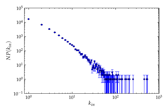
In-degree distribution of a price network with \(10^5\) nodes.
We can draw the graph to see some other features of its topology. For that we use the graph_draw() function.
g = load_graph("price.xml.gz")
age = g.vertex_properties["age"]

graph_draw(g, output_size=(1000, 1000), vertex_color=age,
           vertex_fill_color=age, vertex_size=1, edge_pen_width=1.2,
           output="price.png")
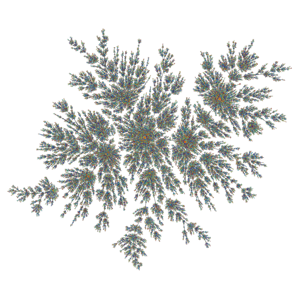
A Price network with \(10^5\) nodes. The vertex colors represent the age of the vertex, from older (red) to newer (blue).
One of the very nice features of graph-tool is the “on-the-fly” filtering of edges and/or vertices. Filtering means the temporary masking of vertices/edges, which are in fact not really removed, and can be easily recovered. Vertices or edges which are to be filtered should be marked with a PropertyMap with value type bool, and then set with set_vertex_filter() or set_edge_filter() methods. By default, vertex or edges with value “1” are kept in the graphs, and those with value “0” are filtered out. This behaviour can be modified with the inverted parameter of the respective functions. All manipulation functions and algorithms will work as if the marked edges or vertices were removed from the graph, with minimum overhead.
Note
It is important to emphasize that the filtering functionality does not add any overhead when the graph is not being filtered. In this case, the algorithms run just as fast as if the filtering functionality didn’t exist.
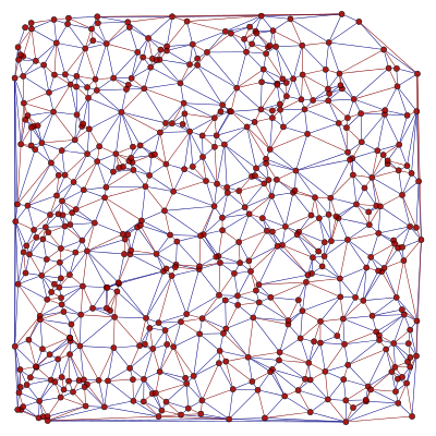
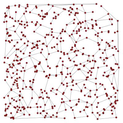
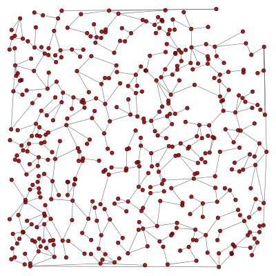
Here is an example which obtains the minimum spanning tree of a graph, using the function min_spanning_tree() and edge filtering.
g, pos = triangulation(random((500, 2)) * 4, type="delaunay")
tree = min_spanning_tree(g)
graph_draw(g, pos=pos, edge_color=tree, output="min_tree.pdf")
The tree property map has a bool type, with value “1” if the edge belongs to the tree, and “0” otherwise. Below is an image of the original graph, with the marked edges.
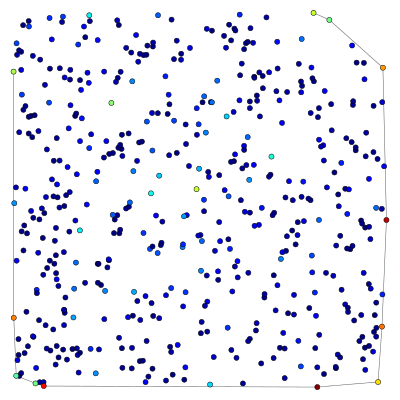
We can now filter out the edges which don’t belong to the minimum spanning tree.
g.set_edge_filter(tree)
graph_draw(g, pos=pos, output="min_tree_filtered.pdf")
This is how the graph looks when filtered:
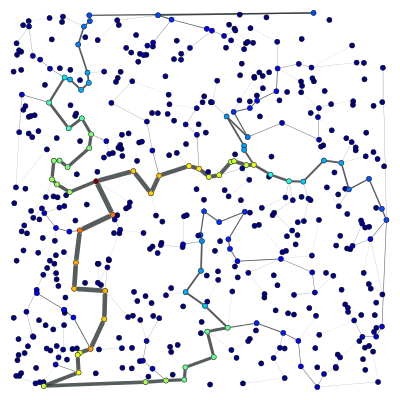
Everything should work transparently on the filtered graph, simply as if the masked edges were removed. For instance, the following code will calculate the betweenness() centrality of the edges and vertices, and draws them as colors and line thickness in the graph.
bv, be = betweenness(g)
be.a /= be.a.max() / 5
graph_draw(g, pos=pos, vertex_fill_color=bv, edge_pen_width=be,
           output="filtered-bt.pdf")
The original graph can be recovered by setting the edge filter to None.
g.set_edge_filter(None)
bv, be = betweenness(g)
be.a /= be.a.max() / 5
graph_draw(g, pos=pos, vertex_fill_color=bv, edge_pen_width=be,
           output="nonfiltered-bt.pdf")
Everything works in analogous fashion with vertex filtering.
Additionally, the graph can also have its edges reversed with the set_reversed() method. This is also an \(O(1)\) operation, which does not really modify the graph.
As mentioned previously, the directedness of the graph can also be changed “on-the-fly” with the set_directed() method.
It is often desired to work with filtered and unfiltered graphs simultaneously, or to temporarily create a filtered version of graph for some specific task. For these purposes, graph-tool provides a GraphView class, which represents a filtered “view” of a graph, and behaves as an independent graph object, which shares the underlying data with the original graph. Graph views are constructed by instantiating a GraphView class, and passing a graph object which is supposed to be filtered, together with the desired filter parameters. For example, to create a directed view of the graph g constructed above, one should do:
>>> ug = GraphView(g, directed=True)
>>> ug.is_directed()
True
Graph views also provide a much more direct and convenient approach to vertex/edge filtering: To construct a filtered minimum spanning tree like in the example above, one must only pass the filter property as the “efilter” parameter:
>>> tv = GraphView(g, efilt=tree)
Note that this is an \(O(1)\) operation, since it is equivalent (in speed) to setting the filter in graph g directly, but in this case the object g remains unmodified.
Like above, the result should be the isolated minimum spanning tree:
>>> bv, be = betweenness(tv)
>>> be.a /= be.a.max() / 5
>>> graph_draw(tv, pos=pos, vertex_fill_color=bv,
...            edge_pen_width=be, output="mst-view.pdf")
<...>

A view of the Delaunay graph, isolating only the minimum spanning tree.
Note
GraphView objects behave exactly like regular Graph objects. In fact, GraphView is a subclass of Graph. The only difference is that a GraphView object shares its internal data with its parent Graph class. Therefore, if the original Graph object is modified, this modification will be reflected immediately in the GraphView object, and vice-versa.
For even more convenience, one can supply a function as filter parameter, which takes a vertex or an edge as single parameter, and returns True if the vertex/edge should be kept and False otherwise. For instance, if we want to keep only the most “central” edges, we can do:
>>> bv, be = betweenness(g)
>>> u = GraphView(g, efilt=lambda e: be[e] > be.a.max() / 2)
This creates a graph view u which contains only the edges of g which have a normalized betweenness centrality larger than half of the maximum value. Note that, differently from the case above, this is an \(O(E)\) operation, where \(E\) is the number of edges, since the supplied function must be called \(E\) times to construct a filter property map. Thus, supplying a constructed filter map is always faster, but supplying a function can be more convenient.
The graph view constructed above can be visualized as
>>> be.a /= be.a.max() / 5
>>> graph_draw(u, pos=pos, vertex_fill_color=bv, output="central-edges-view.pdf")
<...>
A view of the Delaunay graph, isolating only the edges with normalized betweenness centrality larger than 0.01.
Since graph views are regular graphs, one can just as easily create graph views of graph views. This provides a convenient way of composing filters. For instance, in order to isolate the minimum spanning tree of all vertices of the example above which have a degree larger than four, one can do:
>>> u = GraphView(g, vfilt=lambda v: v.out_degree() > 4)
>>> tree = min_spanning_tree(u)
>>> u = GraphView(u, efilt=tree)
The resulting graph view can be visualized as
>>> graph_draw(u, pos=pos, output="composed-filter.pdf")
<...>
A composed view, obtained as the minimum spanning tree of all vertices in the graph which have a degree larger than four.