| shortest_distance | Calculate the distance from a source to a target vertex, or to of all vertices from a given source, or the all pairs shortest paths, if the source is not specified. |
| shortest_path | Return the shortest path from source to target. |
| pseudo_diameter | Compute the pseudo-diameter of the graph. |
| similarity | Return the adjacency similarity between the two graphs. |
| isomorphism | Check whether two graphs are isomorphic. |
| subgraph_isomorphism | Obtain all subgraph isomorphisms of sub in g (or at most max_n subgraphs, if max_n > 0). |
| mark_subgraph | Mark a given subgraph sub on the graph g. |
| max_cardinality_matching | Find a maximum cardinality matching in the graph. |
| max_independent_vertex_set | Find a maximal independent vertex set in the graph. |
| min_spanning_tree | Return the minimum spanning tree of a given graph. |
| random_spanning_tree | Return a random spanning tree of a given graph, which can be directed or undirected. |
| dominator_tree | Return a vertex property map the dominator vertices for each vertex. |
| topological_sort | Return the topological sort of the given graph. |
| transitive_closure | Return the transitive closure graph of g. |
| tsp_tour | Return a traveling salesman tour of the graph, which is guaranteed to be twice as long as the optimal tour in the worst case. |
| sequential_vertex_coloring | Returns a vertex coloring of the graph. |
| label_components | Label the components to which each vertex in the graph belongs. |
| label_biconnected_components | Label the edges of biconnected components, and the vertices which are articulation points. |
| label_largest_component | Label the largest component in the graph. |
| label_out_component | Label the out-component (or simply the component for undirected graphs) of a root vertex. |
| kcore_decomposition | Perform a k-core decomposition of the given graph. |
| is_bipartite | Test if the graph is bipartite. |
| is_DAG | Return True if the graph is a directed acyclic graph (DAG). |
| is_planar | Test if the graph is planar. |
| make_maximal_planar | Add edges to the graph to make it maximally planar. |
| edge_reciprocity | Calculate the edge reciprocity of the graph. |
Return the adjacency similarity between the two graphs.
| Parameters : | g1 : Graph
g2 : Graph
label1 : PropertyMap (optional, default: None)
label2 : PropertyMap (optional, default: None)
norm : bool (optional, default: True)
|
|---|---|
| Returns : | similarity : float
|
Notes
The adjacency similarity is the sum of equal entries in the adjacency matrix, given a vertex ordering determined by the vertex labels. In other words it counts the number of edges which have the same source and target labels in both graphs.
The algorithm runs with complexity \(O(E_1 + V_1 + E_2 + V_2)\).
Examples
>>> g = gt.random_graph(100, lambda: (3,3))
>>> u = g.copy()
>>> gt.similarity(u, g)
1.0
>>> gt.random_rewire(u)
21
>>> gt.similarity(u, g)
0.03
Check whether two graphs are isomorphic.
If isomap is True, a vertex PropertyMap with the isomorphism mapping is returned as well.
Examples
>>> g = gt.random_graph(100, lambda: (3,3))
>>> g2 = gt.Graph(g)
>>> gt.isomorphism(g, g2)
True
>>> g.add_edge(g.vertex(0), g.vertex(1))
<...>
>>> gt.isomorphism(g, g2)
False
Obtain all subgraph isomorphisms of sub in g (or at most max_n subgraphs, if max_n > 0).
| Parameters : | sub : Graph
g : Graph
max_n : int (optional, default: 0)
random : bool (optional, default: False)
|
|---|---|
| Returns : | vertex_maps : list of PropertyMap objects
edge_maps : list of PropertyMap objects
|
Notes
The algorithm used is described in [ullmann-algorithm-1976]. It has a worse-case complexity of \(O(N_g^{N_{sub}})\), but for random graphs it typically has a complexity of \(O(N_g^\gamma)\) with \(\gamma\) depending sub-linearly on the size of sub.
References
| [ullmann-algorithm-1976] | (1, 2) Ullmann, J. R., “An algorithm for subgraph isomorphism”, Journal of the ACM 23 (1): 31-42, 1976, DOI: 10.1145/321921.321925 |
| [subgraph-isormophism-wikipedia] | http://en.wikipedia.org/wiki/Subgraph_isomorphism_problem |
Examples
>>> from numpy.random import poisson
>>> g = gt.random_graph(30, lambda: (poisson(6.1), poisson(6.1)))
>>> sub = gt.random_graph(10, lambda: (poisson(1.9), poisson(1.9)))
>>> vm, em = gt.subgraph_isomorphism(sub, g)
>>> print(len(vm))
35
>>> for i in range(len(vm)):
...   g.set_vertex_filter(None)
...   g.set_edge_filter(None)
...   vmask, emask = gt.mark_subgraph(g, sub, vm[i], em[i])
...   g.set_vertex_filter(vmask)
...   g.set_edge_filter(emask)
...   assert(gt.isomorphism(g, sub))
>>> g.set_vertex_filter(None)
>>> g.set_edge_filter(None)
>>> ewidth = g.copy_property(emask, value_type="double")
>>> ewidth.a += 0.5
>>> ewidth.a *= 2
>>> gt.graph_draw(g, vertex_fill_color=vmask, edge_color=emask,
...               edge_pen_width=ewidth, output_size=(200, 200),
...               output="subgraph-iso-embed.pdf")
<...>
>>> gt.graph_draw(sub, output_size=(200, 200), output="subgraph-iso.pdf")
<...>
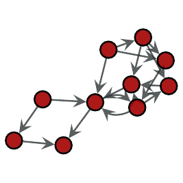
Left: Subgraph searched, Right: One isomorphic subgraph found in main graph.
Mark a given subgraph sub on the graph g.
The mapping must be provided by the vmap and emap parameters, which map vertices/edges of sub to indexes of the corresponding vertices/edges in g.
This returns a vertex and an edge property map, with value type ‘bool’, indicating whether or not a vertex/edge in g corresponds to the subgraph sub.
Return the minimum spanning tree of a given graph.
| Parameters : | g : Graph
weights : PropertyMap (optional, default: None)
root : Vertex (optional, default: None)
tree_map : PropertyMap (optional, default: None)
|
|---|---|
| Returns : | tree_map : PropertyMap
|
Notes
The algorithm runs with \(O(E\log E)\) complexity, or \(O(E\log V)\) if root is specified.
References
| [kruskal-shortest-1956] | J. B. Kruskal. “On the shortest spanning subtree of a graph and the traveling salesman problem”, In Proceedings of the American Mathematical Society, volume 7, pages 48-50, 1956. DOI: 10.1090/S0002-9939-1956-0078686-7 |
| [prim-shortest-1957] | R. Prim. “Shortest connection networks and some generalizations”, Bell System Technical Journal, 36:1389-1401, 1957. |
| [boost-mst] | http://www.boost.org/libs/graph/doc/graph_theory_review.html#sec:minimum-spanning-tree |
| [mst-wiki] | http://en.wikipedia.org/wiki/Minimum_spanning_tree |
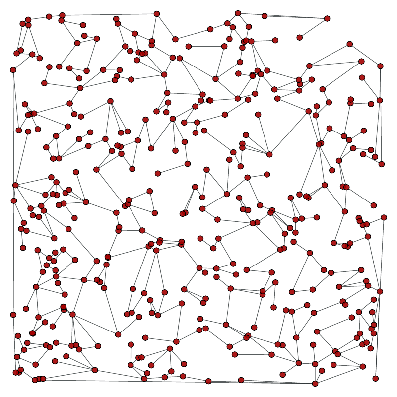
Examples
>>> from numpy.random import random
>>> g, pos = gt.triangulation(random((400, 2)) * 10, type="delaunay")
>>> weight = g.new_edge_property("double")
>>> for e in g.edges():
...    weight[e] = linalg.norm(pos[e.target()].a - pos[e.source()].a)
>>> tree = gt.min_spanning_tree(g, weights=weight)
>>> gt.graph_draw(g, pos=pos, output="triang_orig.pdf")
<...>
>>> g.set_edge_filter(tree)
>>> gt.graph_draw(g, pos=pos, output="triang_min_span_tree.pdf")
<...>
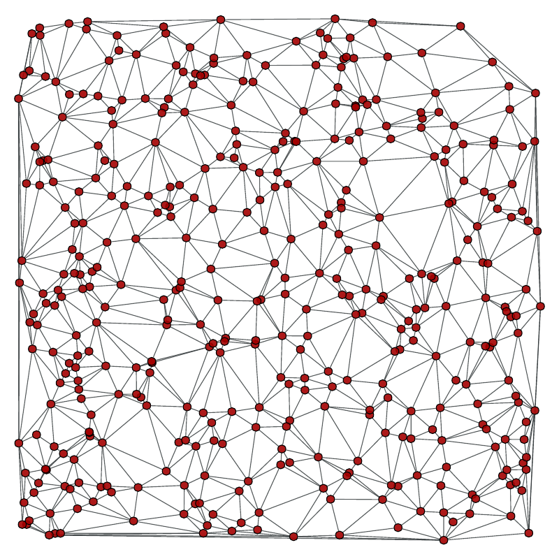
Left: Original graph, Right: The minimum spanning tree.
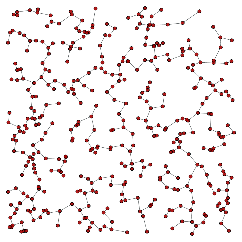
Return a random spanning tree of a given graph, which can be directed or undirected.
| Parameters : | g : Graph
weights : PropertyMap (optional, default: None)
root : Vertex (optional, default: None)
tree_map : PropertyMap (optional, default: None)
|
|---|---|
| Returns : | tree_map : PropertyMap
|
Notes
The typical running time for random graphs is \(O(N\log N)\).
References
| [wilson-generating-1996] | David Bruce Wilson, “Generating random spanning trees more quickly than the cover time”, Proceedings of the twenty-eighth annual ACM symposium on Theory of computing, Pages 296-303, ACM New York, 1996, DOI: 10.1145/237814.237880 |
| [boost-rst] | http://www.boost.org/libs/graph/doc/random_spanning_tree.html |
Examples
>>> from numpy.random import random
>>> g, pos = gt.triangulation(random((400, 2)) * 10, type="delaunay")
>>> weight = g.new_edge_property("double")
>>> for e in g.edges():
...    weight[e] = linalg.norm(pos[e.target()].a - pos[e.source()].a)
>>> tree = gt.random_spanning_tree(g, weights=weight)
>>> gt.graph_draw(g, pos=pos, output="rtriang_orig.pdf")
<...>
>>> g.set_edge_filter(tree)
>>> gt.graph_draw(g, pos=pos, output="triang_random_span_tree.pdf")
<...>

Left: Original graph, Right: A random spanning tree.
Return a vertex property map the dominator vertices for each vertex.
| Parameters : | g : Graph
root : Vertex
dom_map : PropertyMap (optional, default: None)
|
|---|---|
| Returns : | dom_map : PropertyMap
|
Notes
A vertex u dominates a vertex v, if every path of directed graph from the entry to v must go through u.
The algorithm runs with \(O((V+E)\log (V+E))\) complexity.
References
| [dominator-bgl] | http://www.boost.org/libs/graph/doc/lengauer_tarjan_dominator.htm |
Examples
>>> g = gt.random_graph(100, lambda: (2, 2))
>>> tree = gt.min_spanning_tree(g)
>>> g.set_edge_filter(tree)
>>> root = [v for v in g.vertices() if v.in_degree() == 0]
>>> dom = gt.dominator_tree(g, root[0])
>>> print(dom.a)
[ 0  0  0  0  0  0 62  0  0  0  0  0  0  0  0  0  0  0  0  0  0  0  0  0  0
  0  0  0  0  0  0  0  0  0  0  0  0  0  0  0  0  0  0  0  0  0  0  0  0  0
  0  0  0  0  0  0  0  0  0  0  0  0  0  0  0  0  0  0  0  0  0  0  0  0  0
  0  0  0  0  0  0  0  0  0  0  0  0  0  0  0  0  0  0  0  0  0  0  0  0  0]
Return the topological sort of the given graph. It is returned as an array of vertex indexes, in the sort order.
Notes
The topological sort algorithm creates a linear ordering of the vertices such that if edge (u,v) appears in the graph, then v comes before u in the ordering. The graph must be a directed acyclic graph (DAG).
The time complexity is \(O(V + E)\).
References
| [topological-boost] | http://www.boost.org/libs/graph/doc/topological_sort.html |
| [topological-wiki] | http://en.wikipedia.org/wiki/Topological_sorting |
Examples
>>> g = gt.random_graph(30, lambda: (3, 3))
>>> tree = gt.min_spanning_tree(g)
>>> g.set_edge_filter(tree)
>>> sort = gt.topological_sort(g)
>>> print(sort)
[ 1 14  2  7 17  0  3  4  5  6  8  9 22 10 11 12 13 16 23 27 15 18 19 20 21
 24 25 26 28 29]
Return the transitive closure graph of g.
Notes
The transitive closure of a graph G = (V,E) is a graph G* = (V,E*) such that E* contains an edge (u,v) if and only if G contains a path (of at least one edge) from u to v. The transitive_closure() function transforms the input graph g into the transitive closure graph tc.
The time complexity (worst-case) is \(O(VE)\).
References
| [transitive-boost] | http://www.boost.org/libs/graph/doc/transitive_closure.html |
| [transitive-wiki] | http://en.wikipedia.org/wiki/Transitive_closure |
Examples
>>> g = gt.random_graph(30, lambda: (3, 3))
>>> tc = gt.transitive_closure(g)
Label the components to which each vertex in the graph belongs. If the graph is directed, it finds the strongly connected components.
A property map with the component labels is returned, together with an histogram of component labels.
| Parameters : | g : Graph
vprop : PropertyMap (optional, default: None)
directed : bool (optional, default: None)
attractors : bool (optional, default: False)
|
|---|---|
| Returns : | comp : PropertyMap
hist : ndarray
is_attractor : ndarray
|
Notes
The components are arbitrarily labeled from 0 to N-1, where N is the total number of components.
The algorithm runs in \(O(V + E)\) time.
Examples
>>> g = gt.random_graph(100, lambda: (poisson(2), poisson(2)))
>>> comp, hist, is_attractor = gt.label_components(g, attractors=True)
>>> print(comp.a)
[14 15 14 14 14  5 14 14 18 14 14  8 14 14 13 14 14 21 14 14  7 23 10 14 14
 14 24  4 14 14  0 14 14 14 25 14 14  1 14 26 14 19  9 14 14  3 14 14 27 28
 29 14 14  6 14 14 14 30 14 14 20 14  2 14 22 33 34 14 14 14 35 14 14 16 14
 11 36 37 14 14 31 14 14 17 14 14 14 14 14  0 14 38 39 32 14 12 14 40 14 14]
>>> print(hist)
[ 2  1  1  1  1  1  1  1  1  1  1  1  1  1 59  1  1  1  1  1  1  1  1  1  1
  1  1  1  1  1  1  1  1  1  1  1  1  1  1  1  1]
>>> print(is_attractor)
[ True  True  True False False False  True  True False False False False
  True  True False False False False False False False False  True False
 False False False False False False False False False False False False
 False False False False False]
Label the largest component in the graph. If the graph is directed, then the largest strongly connected component is labelled.
A property map with a boolean label is returned.
| Parameters : | g : Graph
directed : bool (optional, default:None)
|
|---|---|
| Returns : | comp : PropertyMap
|
Notes
The algorithm runs in \(O(V + E)\) time.
Examples
>>> g = gt.random_graph(100, lambda: poisson(1), directed=False)
>>> l = gt.label_largest_component(g)
>>> print(l.a)
[1 0 0 0 0 1 0 0 0 0 0 1 0 0 0 0 1 0 0 0 0 0 0 0 0 0 0 0 0 1 0 0 0 0 0 1 0
 0 0 0 0 0 0 0 0 1 0 0 0 1 0 1 1 1 0 0 0 0 0 0 0 0 0 1 0 0 0 0 0 1 0 0 0 0
 0 0 0 0 1 1 0 0 0 0 0 0 0 0 0 0 0 0 0 0 0 0 0 0 0 1]
>>> u = gt.GraphView(g, vfilt=l)   # extract the largest component as a graph
>>> print(u.num_vertices())
16
Label the out-component (or simply the component for undirected graphs) of a root vertex.
| Parameters : | g : Graph
root : Vertex
|
|---|---|
| Returns : | comp : PropertyMap
|
Notes
The algorithm runs in \(O(V + E)\) time.
Examples
>>> g = gt.random_graph(100, lambda: poisson(2.2), directed=False)
>>> l = gt.label_out_component(g, g.vertex(2))
>>> print(l.a)
[1 1 1 1 0 1 1 1 1 1 1 0 1 1 0 1 1 1 1 1 1 1 0 1 1 1 1 1 1 1 1 0 0 1 1 1 0
 1 1 0 0 1 1 0 1 1 0 0 1 1 1 1 0 1 0 0 1 1 1 1 1 1 1 1 1 0 0 1 0 1 1 1 1 1
 1 1 0 1 1 1 1 1 1 1 1 1 1 1 1 1 1 0 1 1 1 0 1 1 0 0]
The in-component can be obtained by reversing the graph.
>>> l = gt.label_out_component(gt.GraphView(g, reversed=True, directed=True),
...                            g.vertex(1))
>>> print(l.a)
[1 1 1 0 0 1 1 0 1 0 0 0 0 1 0 0 0 1 0 0 1 1 0 0 1 0 1 0 0 0 0 0 0 1 1 0 0
 0 1 0 0 0 1 0 1 1 0 0 0 0 1 1 0 0 0 0 1 0 0 0 1 1 0 1 0 0 0 1 0 0 1 1 0 1
 1 0 0 0 0 1 1 0 1 1 0 1 1 1 0 0 1 0 0 0 0 0 1 0 0 0]
Label the edges of biconnected components, and the vertices which are articulation points.
An edge property map with the component labels is returned, together a boolean vertex map marking the articulation points, and an histogram of component labels.
| Parameters : | g : Graph
eprop : PropertyMap (optional, default: None)
vprop : PropertyMap (optional, default: None)
|
|---|---|
| Returns : | bicomp : PropertyMap
articulation : PropertyMap
nc : int
|
Notes
A connected graph is biconnected if the removal of any single vertex (and all edges incident on that vertex) can not disconnect the graph. More generally, the biconnected components of a graph are the maximal subsets of vertices such that the removal of a vertex from a particular component will not disconnect the component. Unlike connected components, vertices may belong to multiple biconnected components: those vertices that belong to more than one biconnected component are called “articulation points” or, equivalently, “cut vertices”. Articulation points are vertices whose removal would increase the number of connected components in the graph. Thus, a graph without articulation points is biconnected. Vertices can be present in multiple biconnected components, but each edge can only be contained in a single biconnected component.
The algorithm runs in \(O(V + E)\) time.
Examples
>>> g = gt.random_graph(100, lambda: poisson(2), directed=False)
>>> comp, art, hist = gt.label_biconnected_components(g)
>>> print(comp.a)
[51 51 51 51 51 51 11 52 51 51 44 42 41 45 49 23 19 51 51 32 38 51 24 37 51
 51 51 10  8 51 20 43 51 51 51 51 51 47 46 51 51 13 14 51 51 51 51 33 30 51
  1 21 51 51 51 35 36  6 51 26 27  7 12  4  3 29 28 51 51 51 31 51 51  0 39
 51 51 51 34 40 51 51  9 17 51 51 18 15 22  2 16 50  5 48 51 51 53 51 51 25]
>>> print(art.a)
[1 0 1 0 0 1 0 0 1 1 0 0 1 1 0 0 0 0 0 0 1 0 0 0 1 0 1 0 0 0 1 0 0 0 1 1 0
 0 1 0 0 1 1 0 1 1 0 0 0 1 1 0 1 1 0 0 0 1 0 0 1 0 1 0 0 1 1 0 0 0 0 0 1 1
 1 0 1 1 0 1 0 1 1 0 0 0 0 1 0 1 0 0 0 1 0 0 0 1 0 0]
>>> print(hist)
[ 1  1  1  1  1  1  1  1  1  1  1  1  1  1  1  1  1  1  1  1  1  1  1  1  1
  1  1  1  1  1  1  1  1  1  1  1  1  1  1  1  1  1  1  1  1  1  1  1  1  1
  1 47  1  1]
Perform a k-core decomposition of the given graph.
| Parameters : | g : Graph
deg : string
vprop : PropertyMap (optional, default: None)
|
|---|---|
| Returns : | kval : PropertyMap
|
Notes
The k-core is a maximal set of vertices such that its induced subgraph only contains vertices with degree larger than or equal to k.
This algorithm is described in [batagelk-algorithm] and runs in \(O(V + E)\) time.
References
| [k-core] | http://en.wikipedia.org/wiki/Degeneracy_%28graph_theory%29 |
| [batagelk-algorithm] | (1, 2) V. Batagelj, M. Zaversnik, “An O(m) Algorithm for Cores Decomposition of Networks”, 2003, arXiv: cs/0310049 |
Examples
>>> g = gt.collection.data["netscience"]
>>> g = gt.GraphView(g, vfilt=gt.label_largest_component(g))
>>> kcore = gt.kcore_decomposition(g)
>>> gt.graph_draw(g, pos=g.vp["pos"], vertex_fill_color=kcore, vertex_text=kcore, output="netsci-kcore.pdf")
<...>
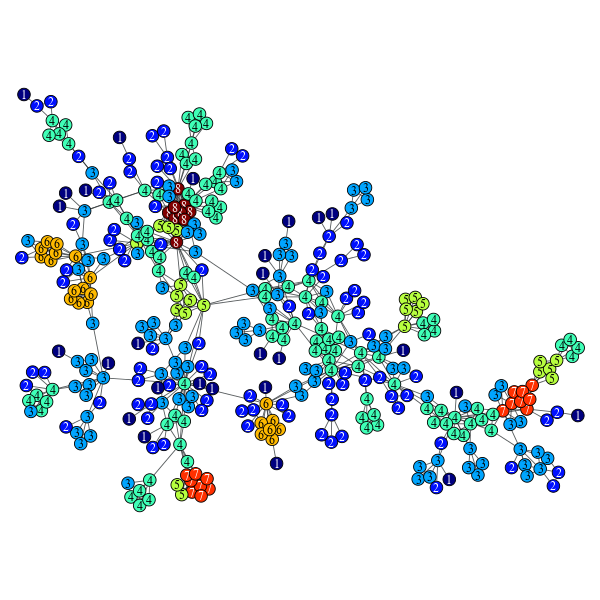
K-core decomposition of a network of network scientists.
Calculate the distance from a source to a target vertex, or to of all vertices from a given source, or the all pairs shortest paths, if the source is not specified.
| Parameters : | g : Graph
source : Vertex (optional, default: None)
target : Vertex (optional, default: None)
weights : PropertyMap (optional, default: None)
max_dist : scalar value (optional, default: None)
directed : bool (optional, default:None)
dense : bool (optional, default: False)
dist_map : PropertyMap (optional, default: None)
pred_map : bool (optional, default: False)
|
|---|---|
| Returns : | dist_map : PropertyMap
|
Notes
If a source is given, the distances are calculated with a breadth-first search (BFS) or Dijkstra’s algorithm [dijkstra], if weights are given. If source is not given, the distances are calculated with Johnson’s algorithm [johnson-apsp]. If dense=True, the Floyd-Warshall algorithm [floyd-warshall-apsp] is used instead.
If source is specified, the algorithm runs in \(O(V + E)\) time, or \(O(V \log V)\) if weights are given. If source is not specified, it runs in \(O(VE\log V)\) time, or \(O(V^3)\) if dense == True.
References
| [bfs] | Edward Moore, “The shortest path through a maze”, International Symposium on the Theory of Switching (1959), Harvard University Press; |
| [bfs-boost] | http://www.boost.org/libs/graph/doc/breadth_first_search.html |
| [dijkstra] | E. Dijkstra, “A note on two problems in connexion with graphs.” Numerische Mathematik, 1:269-271, 1959. |
| [dijkstra-boost] | http://www.boost.org/libs/graph/doc/dijkstra_shortest_paths.html |
| [johnson-apsp] | (1, 2) http://www.boost.org/libs/graph/doc/johnson_all_pairs_shortest.html |
| [floyd-warshall-apsp] | (1, 2) http://www.boost.org/libs/graph/doc/floyd_warshall_shortest.html |
Examples
>>> from numpy.random import poisson
>>> g = gt.random_graph(100, lambda: (poisson(3), poisson(3)))
>>> dist = gt.shortest_distance(g, source=g.vertex(0))
>>> print(dist.a)
[         0          6          3          6 2147483647 2147483647
          6          5          2          4          5          6
          6          3          7          5          4          4
          3          4          2          4          3          3
          4          4          6          6          4          1
          5          2          4          5          3          5
          6          5          4          5 2147483647          9
          4          4          4          6          3          4
          6          6          3          2          4          4
          5          4          5          8          6          6
          5          5          4          5          6          3
          4          3          5          5 2147483647 2147483647
          5          5          8          3          7          4
          5          2          7          5          2          5
          5          5          7          7          4          3
          6          5          5          4          5          5
          4          4          6          5]
>>> dist = gt.shortest_distance(g)
>>> print(dist[g.vertex(0)].a)
[         0          6          3          6 2147483647 2147483647
          6          5          2          4          5          6
          6          3          7          5          4          4
          3          4          2          4          3          3
          4          4          6          6          4          1
          5          2          4          5          3          5
          6          5          4          5 2147483647          9
          4          4          4          6          3          4
          6          6          3          2          4          4
          5          4          5          8          6          6
          5          5          4          5          6          3
          4          3          5          5 2147483647 2147483647
          5          5          8          3          7          4
          5          2          7          5          2          5
          5          5          7          7          4          3
          6          5          5          4          5          5
          4          4          6          5]
Return the shortest path from source to target.
| Parameters : | g : Graph
source : Vertex
target : Vertex
weights : PropertyMap (optional, default: None)
pred_map : PropertyMap (optional, default: None)
|
|---|---|
| Returns : | vertex_list : list of Vertex
edge_list : list of Edge
|
Notes
The paths are computed with a breadth-first search (BFS) or Dijkstra’s algorithm [dijkstra], if weights are given.
The algorithm runs in \(O(V + E)\) time, or \(O(V \log V)\) if weights are given.
References
| [bfs] | Edward Moore, “The shortest path through a maze”, International Symposium on the Theory of Switching (1959), Harvard University Press |
| [bfs-boost] | http://www.boost.org/libs/graph/doc/breadth_first_search.html |
| [dijkstra] | E. Dijkstra, “A note on two problems in connexion with graphs.” Numerische Mathematik, 1:269-271, 1959. |
| [dijkstra-boost] | http://www.boost.org/libs/graph/doc/dijkstra_shortest_paths.html |
Examples
>>> from numpy.random import poisson
>>> g = gt.random_graph(300, lambda: (poisson(4), poisson(4)))
>>> vlist, elist = gt.shortest_path(g, g.vertex(10), g.vertex(11))
>>> print([str(v) for v in vlist])
['10', '131', '184', '265', '223', '11']
>>> print([str(e) for e in elist])
['(10, 131)', '(131, 184)', '(184, 265)', '(265, 223)', '(223, 11)']
Compute the pseudo-diameter of the graph.
| Parameters : | g : Graph
source : Vertex (optional, default: None)
weights : PropertyMap (optional, default: None)
|
|---|---|
| Returns : | pseudo_diameter : int
end_points : pair of Vertex
|
Notes
The pseudo-diameter is an approximate graph diameter. It is obtained by starting from a vertex source, and finds a vertex target that is farthest away from source. This process is repeated by treating target as the new starting vertex, and ends when the graph distance no longer increases. A vertex from the last level set that has the smallest degree is chosen as the final starting vertex u, and a traversal is done to see if the graph distance can be increased. This graph distance is taken to be the pseudo-diameter.
The paths are computed with a breadth-first search (BFS) or Dijkstra’s algorithm [dijkstra], if weights are given.
The algorithm runs in \(O(V + E)\) time, or \(O(V \log V)\) if weights are given.
References
| [pseudo-diameter] | http://en.wikipedia.org/wiki/Distance_%28graph_theory%29 |
Examples
>>> from numpy.random import poisson
>>> g = gt.random_graph(300, lambda: (poisson(3), poisson(3)))
>>> dist, ends = gt.pseudo_diameter(g)
>>> print(dist)
9.0
>>> print(int(ends[0]), int(ends[1]))
0 140
Test if the graph is bipartite.
| Parameters : | g : Graph
partition : bool (optional, default: False)
|
|---|---|
| Returns : | is_bipartite : bool
partition : PropertyMap (only if partition=True)
|
Notes
An undirected graph is bipartite if one can partition its set of vertices into two sets, such that all edges go from one set to the other.
This algorithm runs in \(O(V + E)\) time.
References
| [boost-bipartite] | http://www.boost.org/libs/graph/doc/is_bipartite.html |
Examples
>>> g = gt.lattice([10, 10])
>>> is_bi, part = gt.is_bipartite(g, partition=True)
>>> print(is_bi)
True
>>> gt.graph_draw(g, vertex_fill_color=part, output_size=(300, 300), output="bipartite.pdf")
<...>
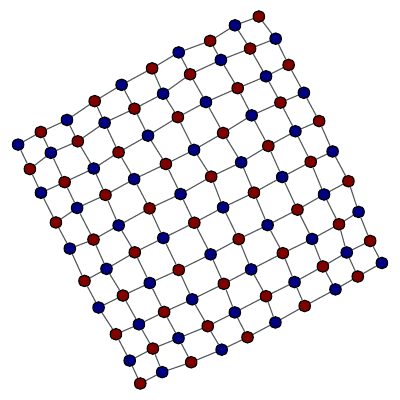
Bipartition of a 2D lattice.
Test if the graph is planar.
| Parameters : | g : Graph
embedding : bool (optional, default: False)
kuratowski : bool (optional, default: False)
|
|---|---|
| Returns : | is_planar : bool
embedding : PropertyMap (only if embedding=True)
kuratowski : PropertyMap (only if kuratowski=True)
|
Notes
A graph is planar if it can be drawn in two-dimensional space without any of its edges crossing. This algorithm performs the Boyer-Myrvold planarity testing [boyer-myrvold]. See [boost-planarity] for more details.
This algorithm runs in \(O(V)\) time.
References
| [boyer-myrvold] | (1, 2) John M. Boyer and Wendy J. Myrvold, “On the Cutting Edge: Simplified O(n) Planarity by Edge Addition” Journal of Graph Algorithms and Applications, 8(2): 241-273, 2004. http://www.emis.ams.org/journals/JGAA/accepted/2004/BoyerMyrvold2004.8.3.pdf |
| [boost-planarity] | http://www.boost.org/libs/graph/doc/boyer_myrvold.html |
Examples
>>> from numpy.random import random
>>> g = gt.triangulation(random((100,2)))[0]
>>> p, embed_order = gt.is_planar(g, embedding=True)
>>> print(p)
True
>>> print(list(embed_order[g.vertex(0)]))
[0, 24, 23, 22, 21, 20, 19, 18, 17, 16, 15, 14, 13, 12, 11, 10, 9, 8, 7, 6, 5, 4, 3, 2, 1]
>>> g = gt.random_graph(100, lambda: 4, directed=False)
>>> p, kur = gt.is_planar(g, kuratowski=True)
>>> print(p)
False
>>> g.set_edge_filter(kur, True)
>>> gt.graph_draw(g, output_size=(300, 300), output="kuratowski.pdf")
<...>
Obstructing Kuratowski subgraph of a random graph.
Add edges to the graph to make it maximally planar.
| Parameters : | g : Graph
|
|---|
Notes
A graph is maximal planar if no additional edges can be added to it without creating a non-planar graph. By Euler’s formula, a maximal planar graph with V > 2 vertices always has 3V - 6 edges and 2V - 4 faces.
The input graph to make_maximal_planar() must be a biconnected planar graph with at least 3 vertices.
This algorithm runs in \(O(V + E)\) time.
References
| [boost-planarity] | http://www.boost.org/libs/graph/doc/make_maximal_planar.html |
Examples
>>> g = gt.lattice([42, 42])
>>> gt.make_maximal_planar(g)
>>> gt.is_planar(g)
True
>>> print(g.num_vertices(), g.num_edges())
1764 5286
>>> gt.graph_draw(g, output_size=(300, 300), output="maximal_planar.pdf")
<...>
A maximally planar graph.
Return True if the graph is a directed acyclic graph (DAG).
Notes
The time complexity is \(O(V + E)\).
References
| [DAG-wiki] | http://en.wikipedia.org/wiki/Directed_acyclic_graph |
Examples
>>> g = gt.random_graph(30, lambda: (3, 3))
>>> print(gt.is_DAG(g))
False
>>> tree = gt.min_spanning_tree(g)
>>> g.set_edge_filter(tree)
>>> print(gt.is_DAG(g))
True
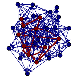
Find a maximum cardinality matching in the graph.
| Parameters : | g : Graph
heuristic : bool (optional, default: False)
weight : PropertyMap (optional, default: None)
minimize : bool (optional, default: True)
match : PropertyMap (optional, default: None)
|
|---|---|
| Returns : | match : PropertyMap
|
Notes
A matching is a subset of the edges of a graph such that no two edges share a common vertex. A maximum cardinality matching has maximum size over all matchings in the graph.
If the parameter weight is provided, as well as heuristic == True a matching with maximum cardinality and maximum (or minimum) weight is returned.
If heuristic == True the algorithm does not necessarily return the maximum matching, instead the focus is to run on linear time.
This algorithm runs in time \(O(EV\times\alpha(E,V))\), where \(\alpha(m,n)\) is a slow growing function that is at most 4 for any feasible input. If heuristic == True, the algorithm runs in time \(O(V + E)\).
For a more detailed description, see [boost-max-matching].
References
| [boost-max-matching] | (1, 2) http://www.boost.org/libs/graph/doc/maximum_matching.html |
| [matching-heuristic] | B. Hendrickson and R. Leland. “A Multilevel Algorithm for Partitioning Graphs.” In S. Karin, editor, Proc. Supercomputing ’95, San Diego. ACM Press, New York, 1995, DOI: 10.1145/224170.224228 |
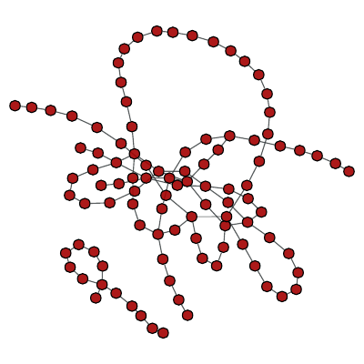
Examples
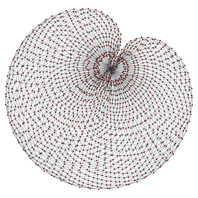
>>> g = gt.GraphView(gt.price_network(300), directed=False)
>>> res = gt.max_cardinality_matching(g)
>>> print(res[1])
True
>>> w = res[0].copy("double")
>>> w.a = 2 * w.a + 2
>>> gt.graph_draw(g, edge_color=res[0], edge_pen_width=w, vertex_fill_color="grey",
...               output="max_card_match.pdf")
<...>
Edges belonging to the matching are in red.
Find a maximal independent vertex set in the graph.
| Parameters : | g : Graph
high_deg : bool (optional, default: False)
mivs : PropertyMap (optional, default: None)
|
|---|---|
| Returns : | mivs : PropertyMap
|
Notes
A maximal independent vertex set is an independent set such that adding any other vertex to the set forces the set to contain an edge between two vertices of the set.
This implements the algorithm described in [mivs-luby], which runs in time \(O(V + E)\).
References
| [mivs-wikipedia] | http://en.wikipedia.org/wiki/Independent_set_%28graph_theory%29 |
| [mivs-luby] | (1, 2) Luby, M., “A simple parallel algorithm for the maximal independent set problem”, Proc. 17th Symposium on Theory of Computing, Association for Computing Machinery, pp. 1-10, (1985) DOI: 10.1145/22145.22146. |
Examples
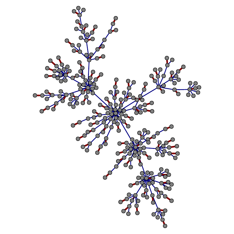
>>> g = gt.GraphView(gt.price_network(300), directed=False)
>>> res = gt.max_independent_vertex_set(g)
>>> gt.graph_draw(g, vertex_fill_color=res, output="mivs.pdf")
<...>
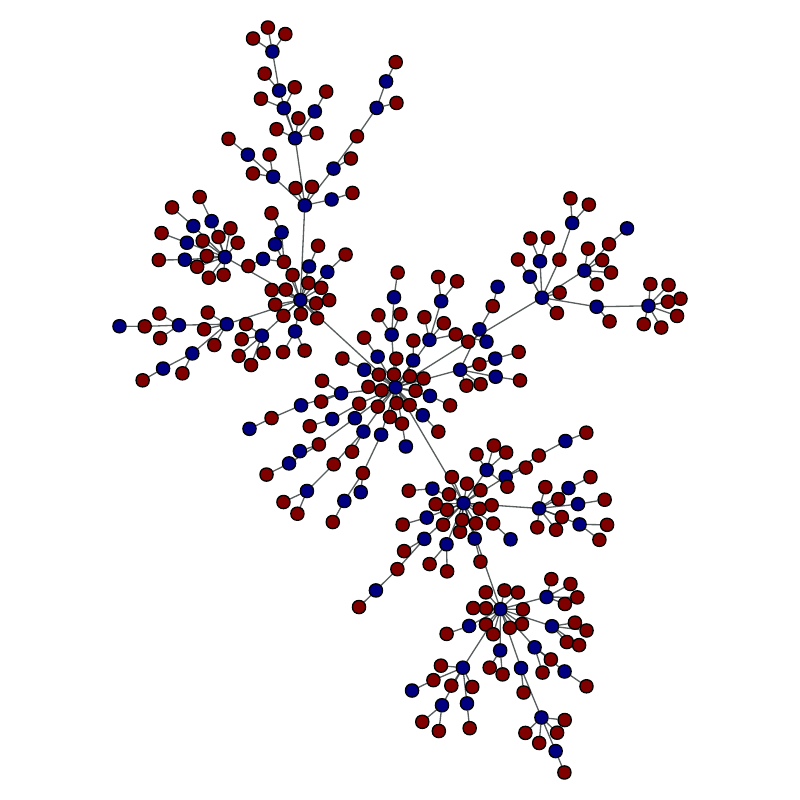
Vertices belonging to the set are in red.
Calculate the edge reciprocity of the graph.
| Parameters : | g : Graph
|
|---|---|
| Returns : | reciprocity : float
|
Notes
The edge [reciprocity] is defined as \(E^\leftrightarrow/E\), where \(E^\leftrightarrow\) and \(E\) are the number of bidirectional and all edges in the graph, respectively.
The algorithm runs with complexity \(O(E + V)\).
References
| [reciprocity] | (1, 2) S. Wasserman and K. Faust, “Social Network Analysis”. (Cambridge University Press, Cambridge, 1994) |
| [lopez-reciprocity-2007] | Gorka Zamora-López, Vinko Zlatić, Changsong Zhou, Hrvoje Štefančić, and Jürgen Kurths “Reciprocity of networks with degree correlations and arbitrary degree sequences”, Phys. Rev. E 77, 016106 (2008) DOI: 10.1103/PhysRevE.77.016106, arXiv: 0706.3372 |
Examples
>>> g = gt.Graph()
>>> g.add_vertex(2)
<...>
>>> g.add_edge(g.vertex(0), g.vertex(1))
<Edge object with source '0' and target '1' at 0x33bc710>
>>> gt.edge_reciprocity(g)
0.0
>>> g.add_edge(g.vertex(1), g.vertex(0))
<Edge object with source '1' and target '0' at 0x33bc7a0>
>>> gt.edge_reciprocity(g)
1.0
Return a traveling salesman tour of the graph, which is guaranteed to be twice as long as the optimal tour in the worst case.
| Parameters : | g : Graph
src : Vertex
weight : PropertyMap (optional, default: None)
|
|---|---|
| Returns : | tour : numpy.ndarray
|
Notes
The algorithm runs with \(O(E\log V)\) complexity.
References
| [tsp-bgl] | http://www.boost.org/libs/graph/doc/metric_tsp_approx.html |
| [tsp] | http://en.wikipedia.org/wiki/Travelling_salesman_problem |
Examples
>>> g = gt.lattice([10, 10])
>>> tour = gt.tsp_tour(g, g.vertex(0))
>>> print(tour)
[ 0  1  2 11 12 21 22 31 32 41 42 51 52 61 62 71 72 81 82 83 73 63 53 43 33
 23 13  3  4  5  6  7  8  9 19 29 39 49 59 69 79 89 14 24 34 44 54 64 74 84
 91 92 93 94 95 85 75 65 55 45 35 25 15 16 17 18 27 28 37 38 47 48 57 58 67
 68 77 78 87 88 97 98 99 26 36 46 56 66 76 86 96 10 20 30 40 50 60 70 80 90
  0]
Returns a vertex coloring of the graph.
| Parameters : | g : Graph
order : PropertyMap (optional, default: None)
color : PropertyMap (optional, default: None)
|
|---|---|
| Returns : | color : PropertyMap
|
Notes
The time complexity is \(O(V(d+k))\), where \(V\) is the number of vertices, \(d\) is the maximum degree of the vertices in the graph, and \(k\) is the number of colors used.
References
| [sgc-bgl] | http://www.boost.org/libs/graph/doc/sequential_vertex_coloring.html |
| [graph-coloring] | http://en.wikipedia.org/wiki/Graph_coloring |
Examples
>>> g = gt.lattice([10, 10])
>>> colors = gt.sequential_vertex_coloring(g)
>>> print(colors.a)
[0 1 0 1 0 1 0 1 0 1 1 0 1 0 1 0 1 0 1 0 0 1 0 1 0 1 0 1 0 1 1 0 1 0 1 0 1
 0 1 0 0 1 0 1 0 1 0 1 0 1 1 0 1 0 1 0 1 0 1 0 0 1 0 1 0 1 0 1 0 1 1 0 1 0
 1 0 1 0 1 0 0 1 0 1 0 1 0 1 0 1 1 0 1 0 1 0 1 0 1 0]