graph_tool.generation - Random graph generation

Summary

random_graph	Generate a random graph, with a given degree distribution and (optionally) vertex-vertex correlation.
random_rewire	Shuffle the graph in-place, following a variety of possible statistical models, chosen via the parameter model.
predecessor_tree	Return a graph from a list of predecessors given by the pred_map vertex property.
line_graph	Return the line graph of the given graph g.
graph_union	Return the union of graphs g1 and g2, composed of all edges and vertices of g1 and g2, without overlap.
triangulation	Generate a 2D or 3D triangulation graph from a given point set.
lattice	Generate a N-dimensional square lattice.
geometric_graph	Generate a geometric network form a set of N-dimensional points.
price_network	A generalized version of Price’s – or Barabási-Albert if undirected – preferential attachment network model.
complete_graph	Generate complete graph.
circular_graph	Generate a circular graph.

Contents

graph_tool.generation.random_graph(N, deg_sampler, directed=True, parallel_edges=False, self_loops=False, block_membership=None, block_type='int', degree_block=False, random=True, verbose=False, **kwargs)

Generate a random graph, with a given degree distribution and (optionally) vertex-vertex correlation.

The graph will be randomized via the random_rewire() function, and any remaining parameters will be passed to that function. Please read its documentation for all the options regarding the different statistical models which can be chosen.

Parameters :

N : int

Number of vertices in the graph.

deg_sampler : function

A degree sampler function which is called without arguments, and returns a tuple of ints representing the in and out-degree of a given vertex (or a single int for undirected graphs, representing the out-degree). This function is called once per vertex, but may be called more times, if the degree sequence cannot be used to build a graph.

Optionally, you can also pass a function which receives one or two arguments. If block_membership == None, the single argument passed will be the index of the vertex which will receive the degree. If block_membership != None, the first value passed will be the vertex index, and the second will be the block value of the vertex.

directed : bool (optional, default: True)

Whether the generated graph should be directed.

parallel_edges : bool (optional, default: False)

If True, parallel edges are allowed.

self_loops : bool (optional, default: False)

If True, self-loops are allowed.

block_membership : list or ndarray or function (optional, default: None)

If supplied, the graph will be sampled from a stochastic blockmodel ensemble, and this parameter specifies the block membership of the vertices, which will be passed to the random_rewire() function.

If the value is a list or a ndarray, it must have len(block_membership) == N, and the values will define to which block each vertex belongs.

If this value is a function, it will be used to sample the block types. It must be callable either with no arguments or with a single argument which will be the vertex index. In either case it must return a type compatible with the block_type parameter.

block_type : string (optional, default: "int")

Value type of block labels. Valid only if block_membership != None.

degree_block : bool (optional, default: False)

If True, the degree of each vertex will be appended to block labels when constructing the blockmodel, such that the resulting block type will be a pair \((r, k)\), where \(r\) is the original block label.

random : bool (optional, default: True)

If True, the returned graph is randomized. Otherwise a deterministic placement of the edges will be used.

verbose : bool (optional, default: False)

If True, verbose information is displayed.

Returns :

random_graph : Graph

The generated graph.

blocks : PropertyMap

A vertex property map with the block values. This is only returned if block_membership != None.

See also

random_rewire

in-place graph shuffling

Notes

The algorithm makes sure the degree sequence is graphical (i.e. realizable) and keeps re-sampling the degrees if is not. With a valid degree sequence, the edges are placed deterministically, and later the graph is shuffled with the random_rewire() function, with all remaining parameters passed to it.

The complexity is \(O(V + E)\) if parallel edges are allowed, and \(O(V + E \times\text{n-iter})\) if parallel edges are not allowed.

Note

If parallel_edges == False this algorithm only guarantees that the returned graph will be a random sample from the desired ensemble if n_iter is sufficiently large. The algorithm implements an efficient Markov chain based on edge swaps, with a mixing time which depends on the degree distribution and correlations desired. If degree correlations are provided, the mixing time tends to be larger.

References

[metropolis-equations-1953]

Metropolis, N.; Rosenbluth, A.W.; Rosenbluth, M.N.; Teller, A.H.; Teller, E. “Equations of State Calculations by Fast Computing Machines”. Journal of Chemical Physics 21 (6): 1087-1092 (1953). DOI: 10.1063/1.1699114

[hastings-monte-carlo-1970]

Hastings, W.K. “Monte Carlo Sampling Methods Using Markov Chains and Their Applications”. Biometrika 57 (1): 97-109 (1970). DOI: 10.1093/biomet/57.1.97

[holland-stochastic-1983]

Paul W. Holland, Kathryn Blackmond Laskey, and Samuel Leinhardt, “Stochastic blockmodels: First steps,” Social Networks 5, no. 2: 109-13 (1983) DOI: 10.1016/0378-8733(83)90021-7

[karrer-stochastic-2011]

Brian Karrer and M. E. J. Newman, “Stochastic blockmodels and community structure in networks,” Physical Review E 83, no. 1: 016107 (2011) DOI: 10.1103/PhysRevE.83.016107 arXiv: 1008.3926

Examples

This is a degree sampler which uses rejection sampling to sample from the distribution \(P(k)\propto 1/k\), up to a maximum.

>>> def sample_k(max):
...     accept = False
...     while not accept:
...         k = randint(1,max+1)
...         accept = random() < 1.0/k
...     return k
...

The following generates a random undirected graph with degree distribution \(P(k)\propto 1/k\) (with k_max=40) and an assortative degree correlation of the form:

\[P(i,k) \propto \frac{1}{1+|i-k|}\]

>>> g = gt.random_graph(1000, lambda: sample_k(40), model="probabilistic",
...                     vertex_corr=lambda i, k: 1.0 / (1 + abs(i - k)), directed=False,
...                     n_iter=100)
>>> gt.scalar_assortativity(g, "out")
(0.6285094791115295, 0.010745128857935755)

The following samples an in,out-degree pair from the joint distribution:

\[p(j,k) = \frac{1}{2}\frac{e^{-m_1}m_1^j}{j!}\frac{e^{-m_1}m_1^k}{k!} + \frac{1}{2}\frac{e^{-m_2}m_2^j}{j!}\frac{e^{-m_2}m_2^k}{k!}\]

with \(m_1 = 4\) and \(m_2 = 20\).

>>> def deg_sample():
...    if random() > 0.5:
...        return poisson(4), poisson(4)
...    else:
...        return poisson(20), poisson(20)
...

The following generates a random directed graph with this distribution, and plots the combined degree correlation.

>>> g = gt.random_graph(20000, deg_sample)
>>>
>>> hist = gt.combined_corr_hist(g, "in", "out")
>>>
>>> clf()
>>> imshow(hist[0].T, interpolation="nearest", origin="lower")
<...>
>>> colorbar()
<...>
>>> xlabel("in-degree")
<...>
>>> ylabel("out-degree")
<...>
>>> savefig("combined-deg-hist.pdf")

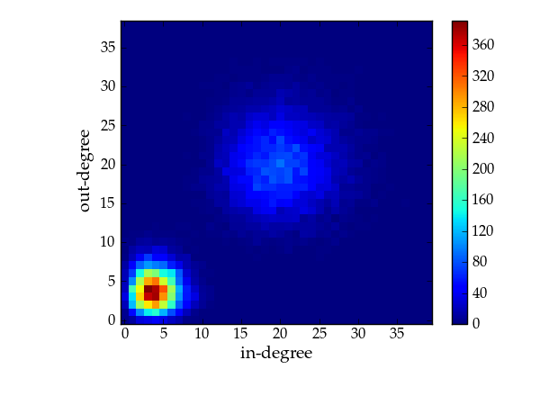
Combined degree histogram.

A correlated directed graph can be build as follows. Consider the following degree correlation:

\[P(j',k'|j,k)=\frac{e^{-k}k^{j'}}{j'!} \frac{e^{-(20-j)}(20-j)^{k'}}{k'!}\]

i.e., the in->out correlation is “disassortative”, the out->in correlation is “assortative”, and everything else is uncorrelated. We will use a flat degree distribution in the range [1,20).

>>> p = scipy.stats.poisson
>>> g = gt.random_graph(20000, lambda: (sample_k(19), sample_k(19)),
...                     model="probabilistic",
...                     vertex_corr=lambda a,b: (p.pmf(a[0], b[1]) *
...                                              p.pmf(a[1], 20 - b[0])),
...                     n_iter=100)

Lets plot the average degree correlations to check.

>>> clf()
>>> axes([0.1,0.15,0.63,0.8])
<...>
>>> corr = gt.avg_neighbour_corr(g, "in", "in")
>>> errorbar(corr[2][:-1], corr[0], yerr=corr[1], fmt="o-",
...         label=r"$\left<\text{in}\right>$ vs in")
<...>
>>> corr = gt.avg_neighbour_corr(g, "in", "out")
>>> errorbar(corr[2][:-1], corr[0], yerr=corr[1], fmt="o-",
...         label=r"$\left<\text{out}\right>$ vs in")
<...>
>>> corr = gt.avg_neighbour_corr(g, "out", "in")
>>> errorbar(corr[2][:-1], corr[0], yerr=corr[1], fmt="o-",
...          label=r"$\left<\text{in}\right>$ vs out")
<...>
>>> corr = gt.avg_neighbour_corr(g, "out", "out")
>>> errorbar(corr[2][:-1], corr[0], yerr=corr[1], fmt="o-",
...          label=r"$\left<\text{out}\right>$ vs out")
<...>
>>> legend(bbox_to_anchor=(1.01, 0.5), loc="center left", borderaxespad=0.)
<...>
>>> xlabel("Source degree")
<...>
>>> ylabel("Average target degree")
<...>
>>> savefig("deg-corr-dir.pdf")

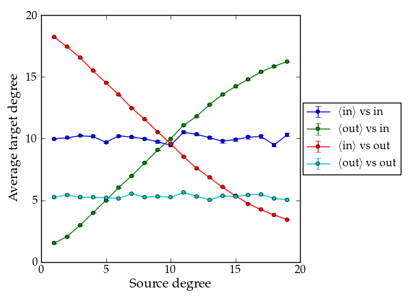
Average nearest neighbour correlations.

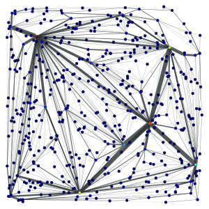
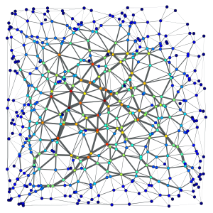
Stochastic blockmodels

The following example shows how a stochastic blockmodel [holland-stochastic-1983] [karrer-stochastic-2011] can be generated. We will consider a system of 10 blocks, which form communities. The connection probability will be given by

>>> def corr(a, b):
...    if a == b:
...        return 0.999
...    else:
...        return 0.001

The blockmodel can be generated as follows.

>>> g, bm = gt.random_graph(5000, lambda: poisson(10), directed=False,
...                         model="blockmodel-traditional",
...                         block_membership=lambda: randint(10),
...                         vertex_corr=corr)
>>> gt.graph_draw(g, vertex_fill_color=bm, edge_color="black", output="blockmodel.pdf")
<...>

Simple blockmodel with 10 blocks.

graph_tool.generation.random_rewire(g, model='uncorrelated', n_iter=1, edge_sweep=True, parallel_edges=False, self_loops=False, vertex_corr=None, block_membership=None, alias=True, cache_probs=True, persist=False, ret_fail=False, verbose=False)

Shuffle the graph in-place, following a variety of possible statistical models, chosen via the parameter model.

Parameters :

g : Graph

Graph to be shuffled. The graph will be modified.

model : string (optional, default: "uncorrelated")

The following statistical models can be chosen, which determine how the edges are rewired.

erdos

The edges will be rewired entirely randomly, and the resulting graph will correspond to the Erdős–Rényi model.

uncorrelated

The edges will be rewired randomly, but the degree sequence of the graph will remain unmodified.

correlated

The edges will be rewired randomly, but both the degree sequence of the graph and the vertex-vertex degree correlations will remain unmodified.

probabilistic

This is similar to the correlated option, but the vertex-vertex correlations are not kept unmodified, but instead are sampled from an arbitrary degree-based probabilistic model specified via the vertex_corr parameter.

blockmodel

This is just like probabilistic, but the values passed to the vertex_corr function will correspond to the block membership values specified by the block_membership parameter.

blockmodel-traditional

This is just like blockmodel, but the degree sequence is not preserved during rewiring.

n_iter : int (optional, default: 1)

Number of iterations. If edge_sweep == True, each iteration corresponds to an entire “sweep” over all edges. Otherwise this corresponds to the total number of edges which are randomly chosen for a swap attempt (which may repeat).

edge_sweep : bool (optional, default: True)

If True, each iteration will perform an entire “sweep” over the edges, where each edge is visited once in random order, and a edge swap is attempted.

parallel : bool (optional, default: False)

If True, parallel edges are allowed.

self_loops : bool (optional, default: False)

If True, self-loops are allowed.

vertex_corr : function (optional, default: None)

A function which gives the vertex-vertex correlation of the graph.

If model == probabilistic it should be callable with two parameters: the (in, out)-degree pair of the source vertex an edge, and the (in,out)-degree pair of the target of the same edge (for undirected graphs, both parameters are single values). The function should return a number proportional to the probability of such an edge existing in the generated graph.

If model == blockmodel or model == blockmodel-traditional, the values passed to the function will be the block value of the respective vertices, as specified via the block_membership. The function should also return a number proportional to the probability of such an edge existing in the generated graph.

block_membership : PropertyMap (optional, default: None)

If supplied, the graph will be rewired to conform to a blockmodel ensemble. The value must be a vertex property map which defines the block of each vertex.

alias : bool (optional, default: True)

If True, and model is any of probabilistic, blockmodel, or blockmodel-traditional, the alias method will be used to sample the candidate edges. In the case of blockmodel-traditional, if parallel_edges == True and self_loops == True this makes the sampling of the edges direct (not rejection based), so that n_iter == 1 is enough to get an uncorrelated sample.

cache_probs : bool (optional, default: True)

If True, the probabilities returned by the vertex_corr parameter will be cached internally. This is crucial for good performance, since in this case the supplied python function is called only a few times, and not at every attempted edge rewire move. However, in the case were the different parameter combinations to the probability function is very large, the memory and time requirements to keep the cache may not be worthwhile.

persist : bool (optional, default: False)

If True, an edge swap which is rejected will be attempted again until it succeeds. This may improve the quality of the shuffling for some probabilistic models, and should be sufficiently fast for sparse graphs, but otherwise it may result in many repeated attempts for certain corner-cases in which edges are difficult to swap.

verbose : bool (optional, default: False)

If True, verbose information is displayed.

Returns :

rejection_count : int

Number of rejected edge moves (due to parallel edges or self-loops, or the probabilistic model used).

See also

random_graph

random graph generation

Notes

This algorithm iterates through all the edges in the network and tries to swap its target or source with the target or source of another edge. The selected canditate swaps are chosen according to the model parameter.

Note

If parallel_edges = False, parallel edges are not placed during rewiring. In this case, the returned graph will be a uncorrelated sample from the desired ensemble only if n_iter is sufficiently large. The algorithm implements an efficient Markov chain based on edge swaps, with a mixing time which depends on the degree distribution and correlations desired. If degree probabilistic correlations are provided, the mixing time tends to be larger.

If model is either “probabilistic” or “blockmodel”, the Markov chain still needs to be mixed, even if parallel edges and self-loops are allowed. In this case the Markov chain is implemented using the Metropolis-Hastings [metropolis-equations-1953] [hastings-monte-carlo-1970] acceptance/rejection algorithm. It will eventually converge to the desired probabilities for sufficiently large values of n_iter.

Each edge is tentatively swapped once per iteration, so the overall complexity is \(O(V + E \times \text{n-iter})\). If edge_sweep == False, the complexity becomes \(O(V + E + \text{n-iter})\).

References

[metropolis-equations-1953]

Metropolis, N.; Rosenbluth, A.W.; Rosenbluth, M.N.; Teller, A.H.; Teller, E. “Equations of State Calculations by Fast Computing Machines”. Journal of Chemical Physics 21 (6): 1087-1092 (1953). DOI: 10.1063/1.1699114

[hastings-monte-carlo-1970]

Hastings, W.K. “Monte Carlo Sampling Methods Using Markov Chains and Their Applications”. Biometrika 57 (1): 97-109 (1970). DOI: 10.1093/biomet/57.1.97

[holland-stochastic-1983]

Paul W. Holland, Kathryn Blackmond Laskey, and Samuel Leinhardt, “Stochastic blockmodels: First steps,” Social Networks 5, no. 2: 109-13 (1983) DOI: 10.1016/0378-8733(83)90021-7

[karrer-stochastic-2011]

Brian Karrer and M. E. J. Newman, “Stochastic blockmodels and community structure in networks,” Physical Review E 83, no. 1: 016107 (2011) DOI: 10.1103/PhysRevE.83.016107 arXiv: 1008.3926

Examples

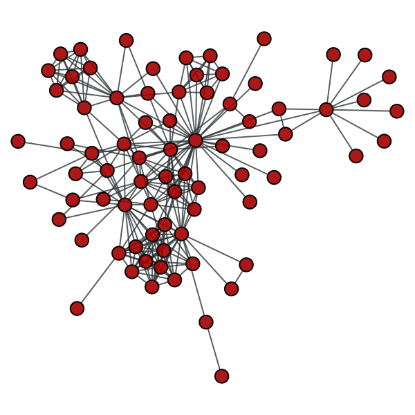
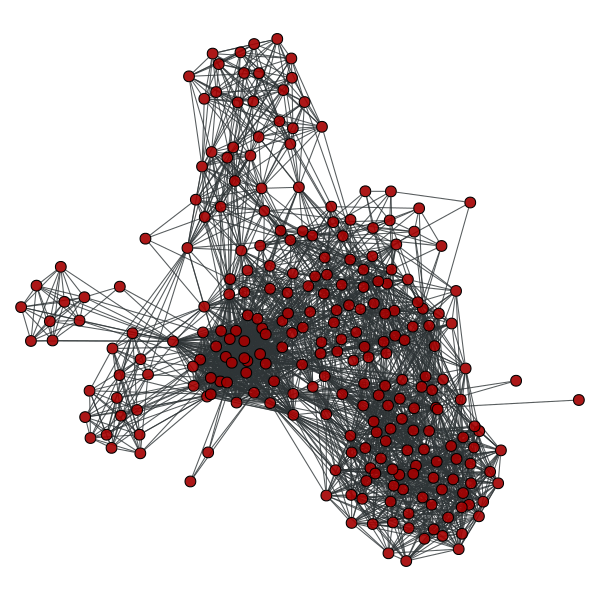
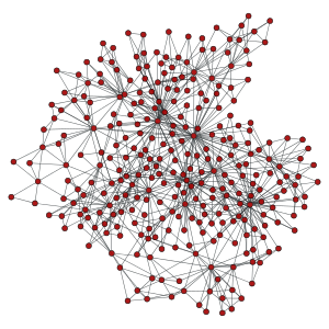
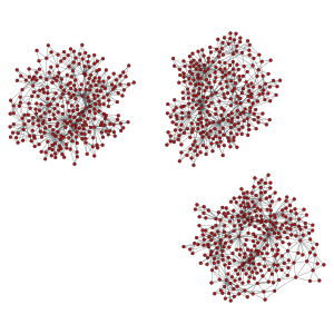
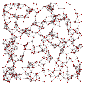
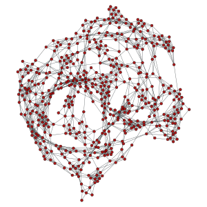
Some small graphs for visualization.

>>> g, pos = gt.triangulation(random((1000,2)))
>>> pos = gt.arf_layout(g)
>>> gt.graph_draw(g, pos=pos, output="rewire_orig.pdf", output_size=(300, 300))
<...>

>>> gt.random_rewire(g, "correlated")
189
>>> pos = gt.arf_layout(g)
>>> gt.graph_draw(g, pos=pos, output="rewire_corr.pdf", output_size=(300, 300))
<...>

>>> gt.random_rewire(g)
197
>>> pos = gt.arf_layout(g)
>>> gt.graph_draw(g, pos=pos, output="rewire_uncorr.pdf", output_size=(300, 300))
<...>

>>> gt.random_rewire(g, "erdos")
26
>>> pos = gt.arf_layout(g)
>>> gt.graph_draw(g, pos=pos, output="rewire_erdos.pdf", output_size=(300, 300))
<...>

Some ridiculograms :

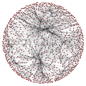
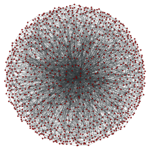
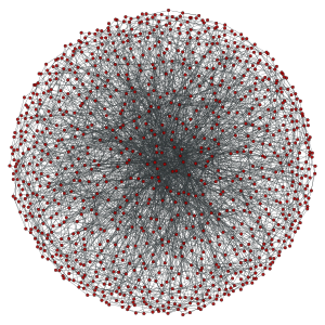
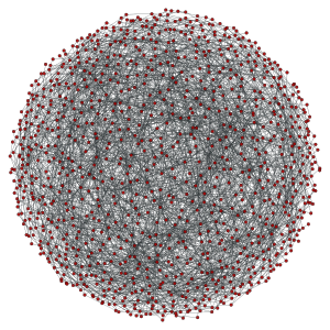
From left to right: Original graph; Shuffled graph, with degree correlations; Shuffled graph, without degree correlations; Shuffled graph, with random degrees.

We can try with larger graphs to get better statistics, as follows.

>>> figure()
<...>
>>> g = gt.random_graph(30000, lambda: sample_k(20), model="probabilistic",
...                     vertex_corr=lambda i, j: exp(abs(i-j)), directed=False,
...                     n_iter=100)
>>> corr = gt.avg_neighbour_corr(g, "out", "out")
>>> errorbar(corr[2][:-1], corr[0], yerr=corr[1], fmt="o-", label="Original")
<...>
>>> gt.random_rewire(g, "correlated")
206
>>> corr = gt.avg_neighbour_corr(g, "out", "out")
>>> errorbar(corr[2][:-1], corr[0], yerr=corr[1], fmt="*", label="Correlated")
<...>
>>> gt.random_rewire(g)
109
>>> corr = gt.avg_neighbour_corr(g, "out", "out")
>>> errorbar(corr[2][:-1], corr[0], yerr=corr[1], fmt="o-", label="Uncorrelated")
<...>
>>> gt.random_rewire(g, "erdos")
13
>>> corr = gt.avg_neighbour_corr(g, "out", "out")
>>> errorbar(corr[2][:-1], corr[0], yerr=corr[1], fmt="o-", label=r"Erd\H{o}s")
<...>
>>> xlabel("$k$")
<...>
>>> ylabel(r"$\left<k_{nn}\right>$")
<...>
>>> legend(loc="best")
<...>
>>> savefig("shuffled-stats.pdf")

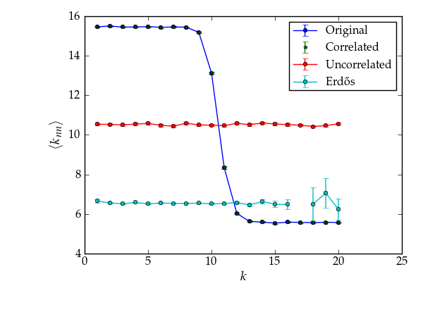
Average degree correlations for the different shuffled and non-shuffled graphs. The shuffled graph with correlations displays exactly the same correlation as the original graph.

Now let’s do it for a directed graph. See random_graph() for more details.

>>> p = scipy.stats.poisson
>>> g = gt.random_graph(20000, lambda: (sample_k(19), sample_k(19)),
...                     model="probabilistic",
...                     vertex_corr=lambda a, b: (p.pmf(a[0], b[1]) * p.pmf(a[1], 20 - b[0])),
...                     n_iter=100)
>>> figure()
<...>
>>> axes([0.1,0.15,0.6,0.8])
<...>
>>> corr = gt.avg_neighbour_corr(g, "in", "out")
>>> errorbar(corr[2][:-1], corr[0], yerr=corr[1], fmt="o-",
...          label=r"$\left<\text{o}\right>$ vs i")
<...>
>>> corr = gt.avg_neighbour_corr(g, "out", "in")
>>> errorbar(corr[2][:-1], corr[0], yerr=corr[1], fmt="o-",
...          label=r"$\left<\text{i}\right>$ vs o")
<...>
>>> gt.random_rewire(g, "correlated")
4323
>>> corr = gt.avg_neighbour_corr(g, "in", "out")
>>> errorbar(corr[2][:-1], corr[0], yerr=corr[1], fmt="o-",
...          label=r"$\left<\text{o}\right>$ vs i, corr.")
<...>
>>> corr = gt.avg_neighbour_corr(g, "out", "in")
>>> errorbar(corr[2][:-1], corr[0], yerr=corr[1], fmt="o-",
...          label=r"$\left<\text{i}\right>$ vs o, corr.")
<...>
>>> gt.random_rewire(g, "uncorrelated")
153
>>> corr = gt.avg_neighbour_corr(g, "in", "out")
>>> errorbar(corr[2][:-1], corr[0], yerr=corr[1], fmt="o-",
...          label=r"$\left<\text{o}\right>$ vs i, uncorr.")
<...>
>>> corr = gt.avg_neighbour_corr(g, "out", "in")
>>> errorbar(corr[2][:-1], corr[0], yerr=corr[1], fmt="o-",
...          label=r"$\left<\text{i}\right>$ vs o, uncorr.")
<...>
>>> legend(bbox_to_anchor=(1.01, 0.5), loc="center left", borderaxespad=0.)
<...>
>>> xlabel("Source degree")
<...>
>>> ylabel("Average target degree")
<...>
>>> savefig("shuffled-deg-corr-dir.pdf")

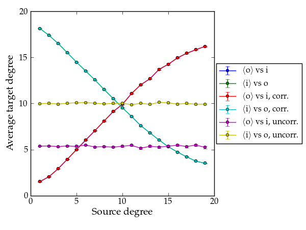
Average degree correlations for the different shuffled and non-shuffled directed graphs. The shuffled graph with correlations displays exactly the same correlation as the original graph.

graph_tool.generation.predecessor_tree(g, pred_map)

Return a graph from a list of predecessors given by the pred_map vertex property.

graph_tool.generation.line_graph(g)

Return the line graph of the given graph g.

Notes

Given an undirected graph G, its line graph L(G) is a graph such that

• each vertex of L(G) represents an edge of G; and
• two vertices of L(G) are adjacent if and only if their corresponding edges share a common endpoint (“are adjacent”) in G.

For a directed graph, the second criterion becomes:

• Two vertices representing directed edges from u to v and from w to x in G are connected by an edge from uv to wx in the line digraph when v = w.

References

[line-wiki]

http://en.wikipedia.org/wiki/Line_graph

Examples

>>> g = gt.collection.data["lesmis"]
>>> lg, vmap = gt.line_graph(g)
>>> gt.graph_draw(g, pos=g.vp["pos"], output="lesmis.pdf")
<...>
>>> pos = gt.graph_draw(lg, output="lesmis-lg.pdf")

Coappearances of characters in Victor Hugo’s novel “Les Miserables”.

Line graph of the coappearance network on the left.

graph_tool.generation.graph_union(g1, g2, intersection=None, props=None, include=False)

Return the union of graphs g1 and g2, composed of all edges and vertices of g1 and g2, without overlap.

Parameters :

g1 : Graph

First graph in the union.

g2 : Graph

Second graph in the union.

intersection : PropertyMap (optional, default: None)

Vertex property map owned by g1 which maps each of each of its vertices to vertex indexes belonging to g2. Negative values mean no mapping exists, and thus both vertices in g1 and g2 will be present in the union graph.

props : list of tuples of PropertyMap (optional, default: [])

Each element in this list must be a tuple of two PropertyMap objects. The first element must be a property of g1, and the second of g2. The values of the property maps are propagated into the union graph, and returned.

include : bool (optional, default: False)

If true, graph g2 is inserted into g1 which is modified. If false, a new graph is created, and both graphs remain unmodified.

Returns :

ug : Graph

The union graph

props : list of PropertyMap objects

List of propagated properties. This is only returned if props is not empty.

Examples

>>> g = gt.triangulation(random((300,2)))[0]
>>> ug = gt.graph_union(g, g)
>>> uug = gt.graph_union(g, ug)
>>> pos = gt.sfdp_layout(g)
>>> gt.graph_draw(g, pos=pos, output_size=(300,300), output="graph_original.pdf")
<...>

>>> pos = gt.sfdp_layout(ug)
>>> gt.graph_draw(ug, pos=pos, output_size=(300,300), output="graph_union.pdf")
<...>

>>> pos = gt.sfdp_layout(uug)
>>> gt.graph_draw(uug, pos=pos, output_size=(300,300), output="graph_union2.pdf")
<...>

graph_tool.generation.triangulation(points, type='simple', periodic=False)

Generate a 2D or 3D triangulation graph from a given point set.

Parameters :

points : ndarray

Point set for the triangulation. It may be either a N x d array, where N is the number of points, and d is the space dimension (either 2 or 3).

type : string (optional, default: 'simple')

Type of triangulation. May be either ‘simple’ or ‘delaunay’.

periodic : bool (optional, default: False)

If True, periodic boundary conditions will be used. This is parameter is valid only for type=”delaunay”, and is otherwise ignored.

Returns :

triangulation_graph : Graph

The generated graph.

pos : PropertyMap

Vertex property map with the Cartesian coordinates.

See also

random_graph

random graph generation

Notes

A triangulation [cgal-triang] is a division of the convex hull of a point set into triangles, using only that set as triangle vertices.

In simple triangulations (type=”simple”), the insertion of a point is done by locating a face that contains the point, and splitting this face into three new faces (the order of insertion is therefore important). If the point falls outside the convex hull, the triangulation is restored by flips. Apart from the location, insertion takes a time O(1). This bound is only an amortized bound for points located outside the convex hull.

Delaunay triangulations (type=”delaunay”) have the specific empty sphere property, that is, the circumscribing sphere of each cell of such a triangulation does not contain any other vertex of the triangulation in its interior. These triangulations are uniquely defined except in degenerate cases where five points are co-spherical. Note however that the CGAL implementation computes a unique triangulation even in these cases.

References

[cgal-triang]

(1, 2) http://www.cgal.org/Manual/last/doc_html/cgal_manual/Triangulation_3/Chapter_main.html

Examples

>>> points = random((500, 2)) * 4
>>> g, pos = gt.triangulation(points)
>>> weight = g.new_edge_property("double") # Edge weights corresponding to
...                                        # Euclidean distances
>>> for e in g.edges():
...    weight[e] = sqrt(sum((array(pos[e.source()]) -
...                          array(pos[e.target()]))**2))
>>> b = gt.betweenness(g, weight=weight)
>>> b[1].a *= 100
>>> gt.graph_draw(g, pos=pos, output_size=(300,300), vertex_fill_color=b[0],
...               edge_pen_width=b[1], output="triang.pdf")
<...>

>>> g, pos = gt.triangulation(points, type="delaunay")
>>> weight = g.new_edge_property("double")
>>> for e in g.edges():
...    weight[e] = sqrt(sum((array(pos[e.source()]) -
...                          array(pos[e.target()]))**2))
>>> b = gt.betweenness(g, weight=weight)
>>> b[1].a *= 120
>>> gt.graph_draw(g, pos=pos, output_size=(300,300), vertex_fill_color=b[0],
...               edge_pen_width=b[1], output="triang-delaunay.pdf")
<...>

2D triangulation of random points:

Left: Simple triangulation. Right: Delaunay triangulation. The vertex colors and the edge thickness correspond to the weighted betweenness centrality.

graph_tool.generation.lattice(shape, periodic=False)

Generate a N-dimensional square lattice.

Parameters :

shape : list or ndarray

List of sizes in each dimension.

periodic : bool (optional, default: False)

If True, periodic boundary conditions will be used.

Returns :

lattice_graph : Graph

The generated graph.

See also

triangulation

2D or 3D triangulation

random_graph

random graph generation

References

[lattice]

http://en.wikipedia.org/wiki/Square_lattice

Examples

>>> g = gt.lattice([10,10])
>>> pos = gt.sfdp_layout(g, cooling_step=0.95, epsilon=1e-2)
>>> gt.graph_draw(g, pos=pos, output_size=(300,300), output="lattice.pdf")
<...>

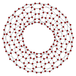
>>> g = gt.lattice([10,20], periodic=True)
>>> pos = gt.sfdp_layout(g, cooling_step=0.95, epsilon=1e-2)
>>> gt.graph_draw(g, pos=pos, output_size=(300,300), output="lattice_periodic.pdf")
<...>

>>> g = gt.lattice([10,10,10])
>>> pos = gt.sfdp_layout(g, cooling_step=0.95, epsilon=1e-2)
>>> gt.graph_draw(g, pos=pos, output_size=(300,300), output="lattice_3d.pdf")
<...>

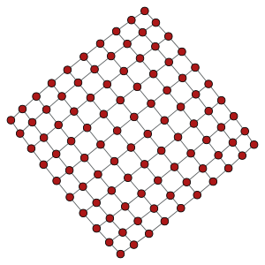
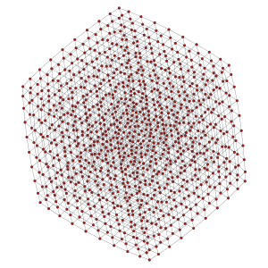
Left: 10x10 2D lattice. Middle: 10x20 2D periodic lattice (torus). Right: 10x10x10 3D lattice.

graph_tool.generation.complete_graph(N, self_loops=False, directed=False)

Generate complete graph.

Parameters :

N : int

Number of vertices.

self_loops : bool (optional, default: False)

If True, self-loops are included.

directed : bool (optional, default: False)

If True, a directed graph is generated.

Returns :

complete_graph : Graph

A complete graph.

References

[complete]

http://en.wikipedia.org/wiki/Complete_graph

Examples

>>> g = gt.complete_graph(30)
>>> pos = gt.sfdp_layout(g, cooling_step=0.95, epsilon=1e-2)
>>> gt.graph_draw(g, pos=pos, output_size=(300,300), output="complete.pdf")
<...>

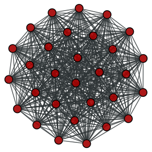
A complete graph with \(N=30\) vertices.

graph_tool.generation.circular_graph(N, k=1, self_loops=False, directed=False)

Generate a circular graph.

Parameters :

N : int

Number of vertices.

k : int (optional, default: True)

Number of nearest neighbours to be connected.

self_loops : bool (optional, default: False)

If True, self-loops are included.

directed : bool (optional, default: False)

If True, a directed graph is generated.

Returns :

circular_graph : Graph

A circular graph.

Examples

>>> g = gt.circular_graph(30, 2)
>>> pos = gt.sfdp_layout(g, cooling_step=0.95)
>>> gt.graph_draw(g, pos=pos, output_size=(300,300), output="circular.pdf")
<...>

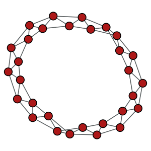
A circular graph with \(N=30\) vertices, and \(k=2\).

graph_tool.generation.geometric_graph(points, radius, ranges=None)

Generate a geometric network form a set of N-dimensional points.

Parameters :

points : list or ndarray

List of points. This must be a two-dimensional array, where the rows are coordinates in a N-dimensional space.

radius : float

Pairs of points with an euclidean distance lower than this parameters will be connected.

ranges : list or ndarray (optional, default: None)

If provided, periodic boundary conditions will be assumed, and the values of this parameter it will be used as the ranges in all dimensions. It must be a two-dimensional array, where each row will cointain the lower and upper bound of each dimension.

Returns :

geometric_graph : Graph

The generated graph.

pos : PropertyMap

A vertex property map with the position of each vertex.

See also

triangulation

2D or 3D triangulation

random_graph

random graph generation

lattice

N-dimensional square lattice

Notes

A geometric graph [geometric-graph] is generated by connecting points embedded in a N-dimensional euclidean space which are at a distance equal to or smaller than a given radius.

References

[geometric-graph]

(1, 2) Jesper Dall and Michael Christensen, “Random geometric graphs”, Phys. Rev. E 66, 016121 (2002), DOI: 10.1103/PhysRevE.66.016121

Examples

>>> points = random((500, 2)) * 4
>>> g, pos = gt.geometric_graph(points, 0.3)
>>> gt.graph_draw(g, pos=pos, output_size=(300,300), output="geometric.pdf")
<...>

>>> g, pos = gt.geometric_graph(points, 0.3, [(0,4), (0,4)])
>>> pos = gt.graph_draw(g, output_size=(300,300), output="geometric_periodic.pdf")

Left: Geometric network with random points. Right: Same network, but

with periodic boundary conditions.

graph_tool.generation.price_network(N, m=1, c=None, gamma=1, directed=True, seed_graph=None)

A generalized version of Price’s – or Barabási-Albert if undirected – preferential attachment network model.

Parameters :

N : int

Size of the network.

m : int (optional, default: 1)

Out-degree of newly added vertices.

c : float (optional, default: 1 if directed == True else 0)

Constant factor added to the probability of a vertex receiving an edge (see notes below).

gamma : float (optional, default: 1)

Preferential attachment power (see notes below).

directed : bool (optional, default: True)

If True, a Price network is generated. If False, a Barabási-Albert network is generated.

seed_graph : Graph (optional, default: None)

If provided, this graph will be used as the starting point of the algorithm.

Returns :

price_graph : Graph

The generated graph.

See also

triangulation

2D or 3D triangulation

random_graph

random graph generation

lattice

N-dimensional square lattice

geometric_graph

N-dimensional geometric network

Notes

The (generalized) [price] network is either a directed or undirected graph (the latter is called a Barabási-Albert network), generated dynamically by at each step adding a new vertex, and connecting it to \(m\) other vertices, chosen with probability \(\pi\) defined as:

\[\pi \propto k^\gamma + c\]

where \(k\) is the in-degree of the vertex (or simply the degree in the undirected case). If \(\gamma=1\), the tail of resulting in-degree distribution of the directed case is given by

\[P_{k_\text{in}} \sim k_\text{in}^{-(2 + c/m)},\]

or for the undirected case

\[P_{k} \sim k^{-(3 + c/m)}.\]

However, if \(\gamma \ne 1\), the in-degree distribution is not scale-free (see [dorogovtsev-evolution] for details).

Note that if seed_graph is not given, the algorithm will always start with one node if \(c > 0\), or with two nodes with a link between them otherwise. If \(m > 1\), the degree of the newly added vertices will be vary dynamically as \(m'(t) = \min(m, N(t))\), where \(N(t)\) is the number of vertices added so far. If this behaviour is undesired, a proper seed graph with \(N \ge m\) vertices must be provided.

This algorithm runs in \(O(N\log N)\) time.

References

[yule]

Yule, G. U. “A Mathematical Theory of Evolution, based on the Conclusions of Dr. J. C. Willis, F.R.S.”. Philosophical Transactions of the Royal Society of London, Ser. B 213: 21-87, 1925, DOI: 10.1098/rstb.1925.0002

[price]

(1, 2) Derek De Solla Price, “A general theory of bibliometric and other cumulative advantage processes”, Journal of the American Society for Information Science, Volume 27, Issue 5, pages 292-306, September 1976, DOI: 10.1002/asi.4630270505

[barabasi-albert]

Barabási, A.-L., and Albert, R., “Emergence of scaling in random networks”, Science, 286, 509, 1999, DOI: 10.1126/science.286.5439.509

[dorogovtsev-evolution]

(1, 2) S. N. Dorogovtsev and J. F. F. Mendes, “Evolution of networks”, Advances in Physics, 2002, Vol. 51, No. 4, 1079-1187, DOI: 10.1080/00018730110112519

Examples

>>> g = gt.price_network(100000)
>>> gt.graph_draw(g, pos=gt.sfdp_layout(g, epsilon=1e-2, cooling_step=0.95),
...               vertex_fill_color=g.vertex_index, vertex_size=2,
...               edge_pen_width=1, output="price-network.png")
<...>
>>> g = gt.price_network(100000, c=0.1)
>>> gt.graph_draw(g, pos=gt.sfdp_layout(g, epsilon=1e-2, cooling_step=0.95),
...               vertex_fill_color=g.vertex_index, vertex_size=2,
...               edge_pen_width=1, output="price-network-broader.png")
<...>

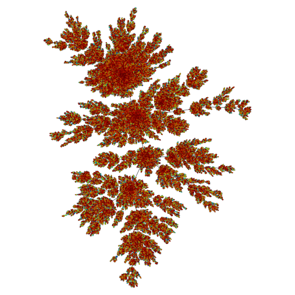
Price network with \(N=10^5\) nodes and \(c=1\). The colors represent the order in which vertices were added.

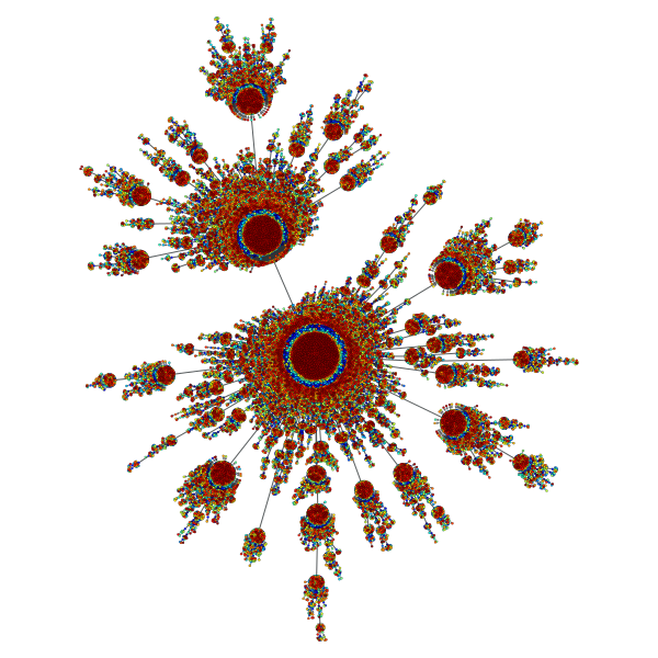
Price network with \(N=10^5\) nodes and \(c=0.1\). The colors represent the order in which vertices were added.