graph_tool.flow - Maximum flow algorithms

Summary

edmonds_karp_max_flow	Calculate maximum flow on the graph with the Edmonds-Karp algorithm.
push_relabel_max_flow	Calculate maximum flow on the graph with the push-relabel algorithm.
boykov_kolmogorov_max_flow	Calculate maximum flow on the graph with the Boykov-Kolmogorov algorithm.
min_st_cut	Get the minimum source-target cut, given the residual capacity of the edges.
min_cut	Get the minimum cut of an undirected graph, given the weight of the edges.

Contents

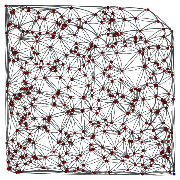
The following network will be used as an example throughout the documentation.

from numpy.random import seed, random
from scipy.linalg import norm
gt.seed_rng(42)
seed(42)
points = random((400, 2))
points[0] = [0, 0]
points[1] = [1, 1]
g, pos = gt.triangulation(points, type="delaunay")
g.set_directed(True)
edges = list(g.edges())
# reciprocate edges
for e in edges:
   g.add_edge(e.target(), e.source())
# The capacity will be defined as the inverse euclidean distance
cap = g.new_edge_property("double")
for e in g.edges():
    cap[e] = min(1.0 / norm(pos[e.target()].a - pos[e.source()].a), 10)
g.edge_properties["cap"] = cap
g.vertex_properties["pos"] = pos
g.save("flow-example.xml.gz")
gt.graph_draw(g, pos=pos, edge_pen_width=gt.prop_to_size(cap, mi=0, ma=3, power=1),
              output="flow-example.pdf")

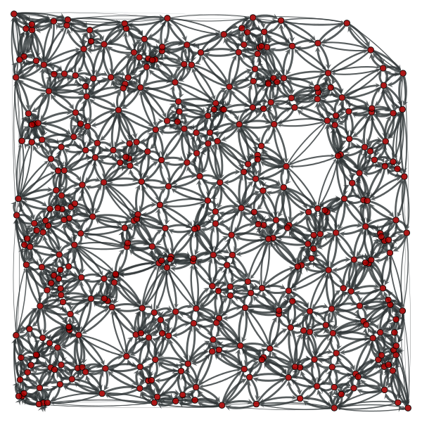
Example network used in the documentation below. The edge capacities are represented by the edge width.

graph_tool.flow.edmonds_karp_max_flow(g, source, target, capacity, residual=None)

Calculate maximum flow on the graph with the Edmonds-Karp algorithm.

Parameters :

g : Graph

Graph to be used.

source : Vertex

The source vertex.

target : Vertex

The target (or “sink”) vertex.

capacity : PropertyMap

Edge property map with the edge capacities.

residual : PropertyMap (optional, default: none)

Edge property map where the residuals should be stored.

Returns :

residual : PropertyMap

Edge property map with the residual capacities (capacity - flow).

Notes

The algorithm is due to [edmonds-theoretical-1972], though we are using the variation called the “labeling algorithm” described in [ravindra-network-1993].

This algorithm provides a very simple and easy to implement solution to the maximum flow problem. However, there are several reasons why this algorithm is not as good as the push_relabel_max_flow() or the boykov_kolmogorov_max_flow() algorithm.

• In the non-integer capacity case, the time complexity is \(O(VE^2)\) which is worse than the time complexity of the push-relabel algorithm \(O(V^2E^{1/2})\) for all but the sparsest of graphs.
• In the integer capacity case, if the capacity bound U is very large then the algorithm will take a long time.

The time complexity is \(O(VE^2)\) in the general case or \(O(VEU)\) if capacity values are integers bounded by some constant \(U\).

References

[boost-edmonds-karp]

http://www.boost.org/libs/graph/doc/edmonds_karp_max_flow.html

[edmonds-theoretical-1972]

(1, 2) Jack Edmonds and Richard M. Karp, “Theoretical improvements in the algorithmic efficiency for network flow problems. Journal of the ACM”, 19:248-264, 1972 DOI: 10.1145/321694.321699

[ravindra-network-1993]

(1, 2) Ravindra K. Ahuja and Thomas L. Magnanti and James B. Orlin,”Network Flows: Theory, Algorithms, and Applications”. Prentice Hall, 1993.

Examples

>>> g = gt.load_graph("flow-example.xml.gz")
>>> cap = g.edge_properties["cap"]
>>> src, tgt = g.vertex(0), g.vertex(1)
>>> res = gt.edmonds_karp_max_flow(g, src, tgt, cap)
>>> res.a = cap.a - res.a  # the actual flow
>>> max_flow = sum(res[e] for e in tgt.in_edges())
>>> print(max_flow)
44.89059578411614
>>> pos = g.vertex_properties["pos"]
>>> gt.graph_draw(g, pos=pos, edge_pen_width=gt.prop_to_size(res, mi=0, ma=5, power=1), output="example-edmonds-karp.pdf")
<...>

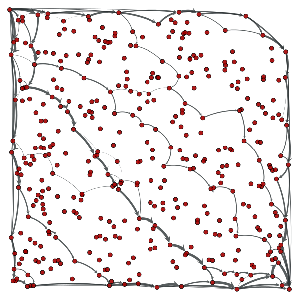
Edge flows obtained with the Edmonds-Karp algorithm. The source and target are on the lower left and upper right corners, respectively. The edge flows are represented by the edge width.

graph_tool.flow.push_relabel_max_flow(g, source, target, capacity, residual=None)

Calculate maximum flow on the graph with the push-relabel algorithm.

Parameters :

g : Graph

Graph to be used.

source : Vertex

The source vertex.

target : Vertex

The target (or “sink”) vertex.

capacity : PropertyMap

Edge property map with the edge capacities.

residual : PropertyMap (optional, default: none)

Edge property map where the residuals should be stored.

Returns :

residual : PropertyMap

Edge property map with the residual capacities (capacity - flow).

Notes

The algorithm is defined in [goldberg-new-1985]. The complexity is \(O(V^3)\).

References

[boost-push-relabel]

http://www.boost.org/libs/graph/doc/push_relabel_max_flow.html

[goldberg-new-1985]

(1, 2) A. V. Goldberg, “A New Max-Flow Algorithm”, MIT Tehnical report MIT/LCS/TM-291, 1985.

Examples

>>> g = gt.load_graph("flow-example.xml.gz")
>>> cap = g.edge_properties["cap"]
>>> src, tgt = g.vertex(0), g.vertex(1)
>>> res = gt.push_relabel_max_flow(g, src, tgt, cap)
>>> res.a = cap.a - res.a  # the actual flow
>>> max_flow = sum(res[e] for e in tgt.in_edges())
>>> print(max_flow)
44.89059578411614
>>> pos = g.vertex_properties["pos"]
>>> gt.graph_draw(g, pos=pos, edge_pen_width=gt.prop_to_size(res, mi=0, ma=5, power=1), output="example-push-relabel.pdf")
<...>

Edge flows obtained with the push-relabel algorithm. The source and target are on the lower left and upper right corners, respectively. The edge flows are represented by the edge width.

graph_tool.flow.boykov_kolmogorov_max_flow(g, source, target, capacity, residual=None)

Calculate maximum flow on the graph with the Boykov-Kolmogorov algorithm.

Parameters :

g : Graph

Graph to be used.

source : Vertex

The source vertex.

target : Vertex

The target (or “sink”) vertex.

capacity : PropertyMap

Edge property map with the edge capacities.

residual : PropertyMap (optional, default: none)

Edge property map where the residuals should be stored.

Returns :

residual : PropertyMap

Edge property map with the residual capacities (capacity - flow).

Notes

The algorithm is defined in [kolmogorov-graph-2003] and [boykov-experimental-2004]. The worst case complexity is \(O(EV^2|C|)\), where \(|C|\) is the minimum cut (but typically performs much better).

For a more detailed description, see [boost-kolmogorov].

References

[boost-kolmogorov]

(1, 2) http://www.boost.org/libs/graph/doc/boykov_kolmogorov_max_flow.html

[kolmogorov-graph-2003]

(1, 2) Vladimir Kolmogorov, “Graph Based Algorithms for Scene Reconstruction from Two or More Views”, PhD thesis, Cornell University, September 2003.

[boykov-experimental-2004]

(1, 2) Yuri Boykov and Vladimir Kolmogorov, “An Experimental Comparison of Min-Cut/Max-Flow Algorithms for Energy Minimization in Vision”, IEEE Transactions on Pattern Analysis and Machine Intelligence, vol. 26, no. 9, pp. 1124-1137, Sept. 2004. DOI: 10.1109/TPAMI.2004.60

Examples

>>> g = gt.load_graph("flow-example.xml.gz")
>>> cap = g.edge_properties["cap"]
>>> src, tgt = g.vertex(0), g.vertex(1)
>>> res = gt.boykov_kolmogorov_max_flow(g, src, tgt, cap)
>>> res.a = cap.a - res.a  # the actual flow
>>> max_flow = sum(res[e] for e in tgt.in_edges())
>>> print(max_flow)
44.89059578411614
>>> pos = g.vertex_properties["pos"]
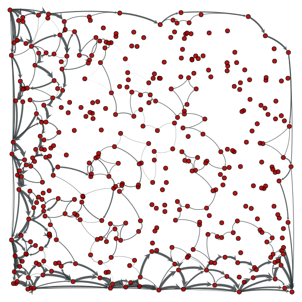
>>> gt.graph_draw(g, pos=pos, edge_pen_width=gt.prop_to_size(res, mi=0, ma=3, power=1), output="example-kolmogorov.pdf")
<...>

Edge flows obtained with the Boykov-Kolmogorov algorithm. The source and target are on the lower left and upper right corners, respectively. The edge flows are represented by the edge width.

graph_tool.flow.min_st_cut(g, source, residual)

Get the minimum source-target cut, given the residual capacity of the edges.

Parameters :

g : Graph

Graph to be used.

source : Vertex

The source vertex.

residual : PropertyMap

Edge property map where the residual capacity is stored.

Returns :

min_cut : float

The value of the minimum cut.

partition : PropertyMap

Boolean-valued vertex property map with the cut partition. Vertices with value True belong to the source side of the cut.

Notes

The source-side of the cut set is obtained by following all vertices which are reachable from the source via edges with nonzero residual capacity.

This algorithm runs in \(O(V+E)\) time.

References

[max-flow-min-cut]

http://en.wikipedia.org/wiki/Max-flow_min-cut_theorem

Examples

>>> g = gt.load_graph("flow-example.xml.gz")
>>> cap = g.edge_properties["cap"]
>>> src, tgt = g.vertex(0), g.vertex(1)
>>> res = gt.boykov_kolmogorov_max_flow(g, src, tgt, cap)
>>> mc, part = gt.min_st_cut(g, src, res)
>>> print(mc)
14.331937627198545
>>> pos = g.vertex_properties["pos"]
>>> res.a = cap.a - res.a  # the actual flow
>>> gt.graph_draw(g, pos=pos, edge_pen_width=gt.prop_to_size(res, mi=0, ma=3, power=1),
...               vertex_fill_color=part, output="example-min-st-cut.pdf")
<...>

Edge flows obtained with the Boykov-Kolmogorov algorithm. The source and target are on the lower left and upper right corners, respectively. The edge flows are represented by the edge width. Vertices of the same color are on the same side of a minimum cut.

graph_tool.flow.min_cut(g, weight)

Get the minimum cut of an undirected graph, given the weight of the edges.

Parameters :

g : Graph

Graph to be used.

weight : PropertyMap

Edge property map with the edge weights.

Returns :

min_cut : float

The value of the minimum cut.

partition : PropertyMap

Boolean-valued vertex property map with the cut partition.

Notes

The algorithm is defined in [stoer_simple_1997].

The time complexity is \(O(VE + V^2 \log V)\).

References

[stoer_simple_1997]

(1, 2) Stoer, Mechthild and Frank Wagner, “A simple min-cut algorithm”. Journal of the ACM 44 (4), 585-591, 1997. DOI: 10.1145/263867.263872

Examples

>>> g = gt.load_graph("mincut-example.xml.gz")
>>> weight = g.edge_properties["weight"]
>>> mc, part = gt.min_cut(g, weight)
>>> print(mc)
4.0
>>> pos = g.vertex_properties["pos"]
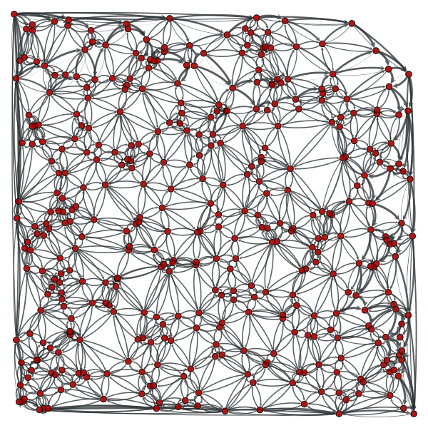
>>> gt.graph_draw(g, pos=pos, edge_pen_width=weight, vertex_fill_color=part,
...               output="example-min-cut.pdf")
<...>

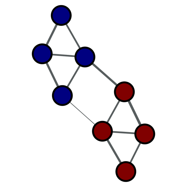
Vertices of the same color are on the same side of a minimum cut. The edge weights are represented by the edge width.