graph_tool.correlations - Correlations

Summary

assortativity	Obtain the assortativity coefficient for the given graph.
scalar_assortativity	Obtain the scalar assortativity coefficient for the given graph.
corr_hist	Obtain the correlation histogram for the given graph.
combined_corr_hist	Obtain the single-vertex combined correlation histogram for the given graph.
avg_neighbour_corr	Obtain the average neighbour-neighbour correlation for the given graph.
avg_combined_corr	Obtain the single-vertex combined correlation histogram for the given graph.

Contents

graph_tool.correlations.assortativity(g, deg)

Obtain the assortativity coefficient for the given graph.

Parameters :

g : Graph

Graph to be used.

deg : string or PropertyMap

degree type (“in”, “out” or “total”) or vertex property map, which specifies the vertex types.

Returns :

assortativity coefficient : tuple of two floats

The assortativity coefficient, and its variance.

See also

assortativity

assortativity coefficient

scalar_assortativity

scalar assortativity coefficient

corr_hist

vertex-vertex correlation histogram

combined_corr_hist

combined single-vertex correlation histogram

avg_neighbour_corr

average nearest-neighbour correlation

avg_combined_corr

average combined single-vertex correlation

Notes

The assortativity coefficient [newman-mixing-2003] tells in a concise fashion how vertices of different types are preferentially connected amongst themselves, and is defined by

\[r = \frac{\sum_i e_{ii} - \sum_i a_i b_i}{1-\sum_i a_i b_i}\]

where \(a_i=\sum_je_{ij}\) and \(b_j=\sum_ie_{ij}\), and \(e_{ij}\) is the fraction of edges from a vertex of type i to a vertex of type j.

The variance is obtained with the jackknife method.

If enabled during compilation, this algorithm runs in parallel.

References

[newman-mixing-2003]

M. E. J. Newman, “Mixing patterns in networks”, Phys. Rev. E 67, 026126 (2003), DOI: 10.1103/PhysRevE.67.026126

Examples

>>> def sample_k(max):
...     accept = False
...     while not accept:
...         k = np.random.randint(1,max+1)
...         accept = random() < 1.0/k
...     return k
...
>>> g = gt.random_graph(1000, lambda: sample_k(40), model="probabilistic",
...                     vertex_corr=lambda i,k: 1.0 / (1 + abs(i - k)), directed=False,
...                     n_iter=100)
>>> gt.assortativity(g, "out")
(0.13903518011375607, 0.005051876804786422)

graph_tool.correlations.scalar_assortativity(g, deg)

Obtain the scalar assortativity coefficient for the given graph.

Parameters :

g : Graph

Graph to be used.

deg : string or PropertyMap

degree type (“in”, “out” or “total”) or vertex property map, which specifies the vertex types.

Returns :

scalar assortativity coefficient : tuple of two floats

The scalar assortativity coefficient, and its variance.

See also

assortativity

assortativity coefficient

scalar_assortativity

scalar assortativity coefficient

corr_hist

vertex-vertex correlation histogram

combined_corr_hist

combined single-vertex correlation histogram

avg_neighbour_corr

average nearest-neighbour correlation

avg_combined_corr

average combined single-vertex correlation

Notes

The scalar assortativity coefficient [newman-mixing-2003] tells in a concise fashion how vertices of different types are preferentially connected amongst themselves, and is defined by

\[r = \frac{\sum_{xy} xy(e_{xy} - a_x b_y)}{\sigma_a\sigma_b}\]

where \(a_x=\sum_ye_{xy}\) and \(b_y=\sum_xe_{xy}\), and \(e_{xy}\) is the fraction of edges from a vertex of type x to a vertex of type y.

The variance is obtained with the jackknife method.

If enabled during compilation, this algorithm runs in parallel.

References

[newman-mixing-2003]

M. E. J. Newman, “Mixing patterns in networks”, Phys. Rev. E 67, 026126 (2003), DOI: 10.1103/PhysRevE.67.026126

Examples

>>> def sample_k(max):
...     accept = False
...     while not accept:
...         k = np.random.randint(1,max+1)
...         accept = random() < 1.0/k
...     return k
...
>>> g = gt.random_graph(1000, lambda: sample_k(40), model="probabilistic",
...                     vertex_corr=lambda i,k: abs(i-k),
...                     directed=False, n_iter=100)
>>> gt.scalar_assortativity(g, "out")
(-0.44070158356400696, 0.010592022444678632)

>>> g = gt.random_graph(1000, lambda: sample_k(40), model="probabilistic",
...                     vertex_corr=lambda i, k: 1.0 / (1 + abs(i - k)),
...                     directed=False, n_iter=100)
>>> gt.scalar_assortativity(g, "out")
(0.6007430887839058, 0.011569809783643956)

graph_tool.correlations.corr_hist(g, deg_source, deg_target, bins=[[0, 1], [0, 1]], weight=None, float_count=True)

Obtain the correlation histogram for the given graph.

Parameters :

g : Graph

Graph to be used.

deg_source : string or PropertyMap

degree type (“in”, “out” or “total”) or vertex property map for the source vertex.

deg_target : string or PropertyMap

degree type (“in”, “out” or “total”) or vertex property map for the target vertex.

bins : list of lists (optional, default: [[0, 1], [0, 1]])

A list of bin edges to be used for the source and target degrees. If any list has size 2, it is used to create an automatically generated bin range starting from the first value, and with constant bin width given by the second value.

weight : edge property map (optional, default: None)

Weight (multiplicative factor) to be used on each edge.

float_count : bool (optional, default: True)

If True, the bin counts are converted float variables, which is useful for normalization, and other processing. It False, the bin counts will be unsigned integers.

Returns :

bin_counts : ndarray

Two-dimensional array with the bin counts.

source_bins : ndarray

Source degree bins

target_bins : ndarray

Target degree bins

See also

assortativity

assortativity coefficient

scalar_assortativity

scalar assortativity coefficient

corr_hist

vertex-vertex correlation histogram

combined_corr_hist

combined single-vertex correlation histogram

avg_neighbour_corr

average nearest-neighbour correlation

avg_combined_corr

average combined single-vertex correlation

Notes

The correlation histogram counts, for every vertex with degree (or scalar property) ‘source_deg’, the number of out-neighbours with degree (or scalar property) ‘target_deg’.

If enabled during compilation, this algorithm runs in parallel.

Examples

>>> def sample_k(max):
...     accept = False
...     while not accept:
...         k = np.random.randint(1,max+1)
...         accept = random() < 1.0/k
...     return k
...
>>> g = gt.random_graph(10000, lambda: sample_k(40), model="probabilistic",
...                     vertex_corr=lambda i, j: (sin(i / pi) * sin(j / pi) + 1) / 2,
...                     directed=False, n_iter=100)
>>> h = gt.corr_hist(g, "out", "out")
>>> clf()
>>> xlabel("Source out-degree")
<...>
>>> ylabel("Target out-degree")
<...>
>>> imshow(h[0].T, interpolation="nearest", origin="lower")
<...>
>>> colorbar()
<...>
>>> savefig("corr.pdf")

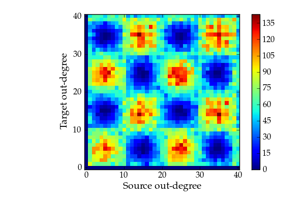
Out/out-degree correlation histogram.

graph_tool.correlations.combined_corr_hist(g, deg1, deg2, bins=[[0, 1], [0, 1]], float_count=True)

Obtain the single-vertex combined correlation histogram for the given graph.

Parameters :

g : Graph

Graph to be used.

deg1 : string or PropertyMap

first degree type (“in”, “out” or “total”) or vertex property map.

deg2 : string or PropertyMap

second degree type (“in”, “out” or “total”) or vertex property map.

bins : list of lists (optional, default: [[0, 1], [0, 1]])

A list of bin edges to be used for the first and second degrees. If any list has size 2, it is used to create an automatically generated bin range starting from the first value, and with constant bin width given by the second value.

float_count : bool (optional, default: True)

If True, the bin counts are converted float variables, which is useful for normalization, and other processing. It False, the bin counts will be unsigned integers.

Returns :

bin_counts : ndarray

Two-dimensional array with the bin counts.

first_bins : ndarray

First degree bins

second_bins : ndarray

Second degree bins

See also

assortativity

assortativity coefficient

scalar_assortativity

scalar assortativity coefficient

corr_hist

vertex-vertex correlation histogram

combined_corr_hist

combined single-vertex correlation histogram

avg_neighbour_corr

average nearest-neighbour correlation

avg_combined_corr

average combined single-vertex correlation

Notes

If enabled during compilation, this algorithm runs in parallel.

Examples

>>> def sample_k(max):
...     accept = False
...     while not accept:
...         i = randint(1, max + 1)
...         j = randint(1, max + 1)
...         accept = random() < (sin(i / pi) * sin(j / pi) + 1) / 2
...     return i,j
...
>>> g = gt.random_graph(10000, lambda: sample_k(40))
>>> h = gt.combined_corr_hist(g, "in", "out")
>>> clf()
>>> xlabel("In-degree")
<...>
>>> ylabel("Out-degree")
<...>
>>> imshow(h[0].T, interpolation="nearest", origin="lower")
<...>
>>> colorbar()
<...>
>>> savefig("combined_corr.pdf")

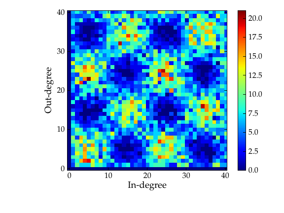
Combined in/out-degree correlation histogram.

graph_tool.correlations.avg_neighbour_corr(g, deg_source, deg_target, bins=[0, 1], weight=None)

Obtain the average neighbour-neighbour correlation for the given graph.

Parameters :

g : Graph

Graph to be used.

deg_source : string or PropertyMap

degree type (“in”, “out” or “total”) or vertex property map for the source vertex.

deg_target : string or PropertyMap

degree type (“in”, “out” or “total”) or vertex property map for the target vertex.

bins : list (optional, default: [0, 1])

Bins to be used for the source degrees. If the list has size 2, it is used as the constant width of an automatically generated bin range, starting from the first value.

weight : edge property map (optional, default: None)

Weight (multiplicative factor) to be used on each edge.

Returns :

bin_avg : ndarray

Array with the deg_target average for the get_source bins.

bin_dev : ndarray

Array with the standard deviation of the deg_target average for the get_source bins.

bins : ndarray

Source degree bins,

See also

assortativity

assortativity coefficient

scalar_assortativity

scalar assortativity coefficient

corr_hist

vertex-vertex correlation histogram

combined_corr_hist

combined single-vertex correlation histogram

avg_neighbour_corr

average nearest-neighbour correlation

avg_combined_corr

average combined single-vertex correlation

Notes

The average correlation is the average, for every vertex with degree (or scalar property) ‘source_deg’, the of the ‘target_deg’ degree (or scalar property) of its neighbours.

If enabled during compilation, this algorithm runs in parallel.

Examples

>>> def sample_k(max):
...     accept = False
...     while not accept:
...         k = randint(1,max+1)
...         accept = random() < 1.0 / k
...     return k
...
>>> g = gt.random_graph(10000, lambda: sample_k(40), model="probabilistic",
...                     vertex_corr=lambda i, j: (sin(i / pi) * sin(j / pi) + 1) / 2,
...                     directed=False, n_iter=100)
>>> h = gt.avg_neighbour_corr(g, "out", "out")
>>> clf()
>>> xlabel("Source out-degree")
<...>
>>> ylabel("Target out-degree")
<...>
>>> errorbar(h[2][:-1], h[0], yerr=h[1], fmt="o")
<...>
>>> savefig("avg_corr.pdf")

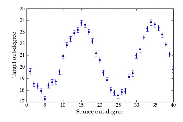
Average out/out degree correlation.

graph_tool.correlations.avg_combined_corr(g, deg1, deg2, bins=[0, 1])

Obtain the single-vertex combined correlation histogram for the given graph.

Parameters :

g : Graph

Graph to be used.

deg1 : string or PropertyMap

first degree type (“in”, “out” or “total”) or vertex property map.

deg2 : string or PropertyMap

second degree type (“in”, “out” or “total”) or vertex property map.

bins : list (optional, default: [0, 1])

Bins to be used for the first degrees. If the list has size 2, it is used as the constant width of an automatically generated bin range, starting from the first value.

Returns :

bin_avg : ndarray

Array with the deg2 average for the deg1 bins.

bin_dev : ndarray

Array with the standard deviation of the deg2 average for the deg1 bins.

bins : ndarray

The deg1 bins.

See also

assortativity

assortativity coefficient

scalar_assortativity

scalar assortativity coefficient

corr_hist

vertex-vertex correlation histogram

combined_corr_hist

combined single-vertex correlation histogram

avg_neighbour_corr

average nearest-neighbour correlation

avg_combined_corr

average combined single-vertex correlation

Notes

If enabled during compilation, this algorithm runs in parallel.

Examples

>>> def sample_k(max):
...     accept = False
...     while not accept:
...         i = randint(1,max+1)
...         j = randint(1,max+1)
...         accept = random() < (sin(i/pi)*sin(j/pi)+1)/2
...     return i,j
...
>>> g = gt.random_graph(10000, lambda: sample_k(40))
>>> h = gt.avg_combined_corr(g, "in", "out")
>>> clf()
>>> xlabel("In-degree")
<...>
>>> ylabel("Out-degree")
<...>
>>> errorbar(h[2][:-1], h[0], yerr=h[1], fmt="o")
<...>
>>> savefig("combined_avg_corr.pdf")

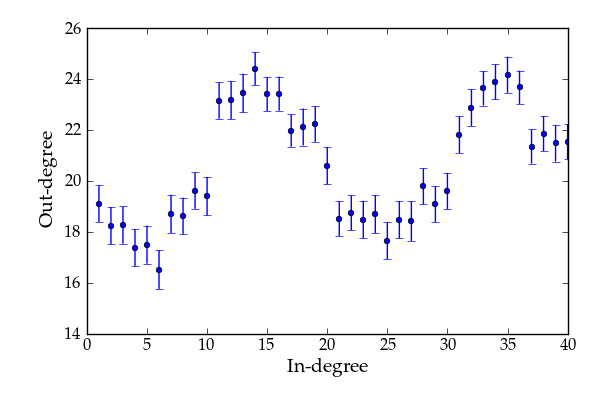
Average combined in/out-degree correlation.