graph_tool.community - Community structure

This module contains algorithms for the computation of community structure on graphs.

Stochastic blockmodel inference

Summary

minimize_blockmodel_dl	Find the block partition of an unspecified size which minimizes the description length of the network, according to the stochastic blockmodel ensemble which best describes it.
BlockState	This class encapsulates the block state of a given graph.
mcmc_sweep	Performs a Monte Carlo Markov chain sweep on the network, to sample the block partition according to a probability \(\propto e^{-\beta \mathcal{S}_{t/c}}\), where \(\mathcal{S}_{t/c}\) is the blockmodel entropy.
collect_vertex_marginals	Collect the vertex marginal histogram, which counts the number of times a node was assigned to a given block.
collect_edge_marginals	Collect the edge marginal histogram, which counts the number of times the endpoints of each node have been assigned to a given block pair.
mf_entropy	Compute the “mean field” entropy given the vertex block membership marginals.
bethe_entropy	Compute the Bethe entropy given the edge block membership marginals.
model_entropy	Computes the amount of information necessary for the parameters of the traditional blockmodel ensemble, for B blocks, N vertices, E edges, and either a directed or undirected graph.
get_max_B	Return the maximum detectable number of blocks, obtained by minimizing: ..
get_akc	Return the minimum value of the average degree of the network, so that some block structure with \(B\) blocks can be detected, according to the minimum description length criterion.
min_dist	Return the minimum distance between all blocks, and the block pair which minimizes it.
condensation_graph	Obtain the condensation graph, where each vertex with the same ‘prop’ value is condensed in one vertex.

Modularity-based community detection

Summary

community_structure	Obtain the community structure for the given graph, using a Potts model approach.
modularity	Calculate Newman’s modularity.

Contents

graph_tool.community.minimize_blockmodel_dl(g, deg_corr=True, nsweeps=100, adaptive_convergence=True, anneal=1.0, greedy_cooling=True, max_B=None, min_B=1, mid_B=None, b_cache=None, b_start=None, clabel=None, checkpoint=None, verbose=False)

Find the block partition of an unspecified size which minimizes the description length of the network, according to the stochastic blockmodel ensemble which best describes it.

Parameters :

g : Graph

Graph being used.

deg_corr : bool (optional, default: True)

If True, the degree-corrected version of the blockmodel ensemble will be assumed, otherwise the traditional variant will be used.

nsweeps : int (optional, default: 50)

Number of sweeps per value of B tried. If adaptive_convergence == True, this corresponds to the number of sweeps observed to determine convergence, not the total number of sweeps performed, which can be much larger.

adaptive_convergence : bool (optional, default: True)

If True, the parameter nsweeps represents not the total number of sweeps performed per value of B, but instead the number of sweeps without an improvement on the value of \(S_{c/t}\) so that convergence is assumed.

anneal : float (optional, default: 1.)

Annealing factor which multiplies the inverse temperature \(\beta\) after each convergence. If anneal <= 1., no annealing is performed.

greedy_cooling : bool (optional, default: True)

If True, a final abrupt cooling step is performed after the Markov chain has equilibrated.

max_B : int (optional, default: None)

Maximum number of blocks tried. If not supplied, it will be automatically determined.

min_B : int (optional, default: 1)

Minimum number of blocks tried.

mid_B : int (optional, default: None)

Middle of the range which brackets the minimum. If not supplied, will be automatically determined.

b_cache : dict with int keys and (float, PropertyMap) values (optional, default: None)

If provided, this corresponds to a dictionary where the keys are the number of blocks, and the values are tuples containing two values: the description length and its associated vertex partition. Values present in this dictionary will not be computed, and will be used unmodified as the solution for the corresponding number of blocks. This can be used to continue from a previously unfinished run.

b_start : dict with int keys and (float, PropertyMap) values (optional, default: None)

Like b_cache, but the partitions present in the dictionary will be used as the starting point of the minimization.

clabel : PropertyMap (optional, default: None)

Constraint labels on the vertices, such that vertices with different labels cannot belong to the same block.

checkpoint : function (optional, default: None)

If provided, this function will be called after each call to mcmc_sweep(). This can be used to store the current state, so it can be continued later. The function must have the following signature:

def checkpoint(state, L, delta, nmoves):
    ...

where state is either a BlockState instance or None, L is the current description length, delta is the entropy difference in the last MCMC sweep, and nmoves is the number of accepted block membership moves.

This function will also be called when the MCMC has finished for the current value of \(B\), in which case state == None, and the remaining parameters will be zero.

verbose : bool (optional, default: False)

If True, verbose information is displayed.

Returns :

b : PropertyMap

Vertex property map with the best block partition.

min_dl : float

Minimum value of the description length (in nats).

b_cache : dict with int keys and (float, PropertyMap) values

Dictionary where the keys are the number of blocks visited during the algorithm, and the values are tuples containing two values: the description length and its associated vertex partition.

Notes

This algorithm attempts to find a block partition of an unspecified size which minimizes the description length of the network,

\[\Sigma_{t/c} = \mathcal{S}_{t/c} + \mathcal{L}_{t/c},\]

where \(\mathcal{S}_{t/c}\) is the blockmodel entropy (as described in the docstring of mcmc_sweep() and BlockState.entropy()) and \(\mathcal{L}_{t/c}\) is the information necessary to describe the model (as described in the docstring of model_entropy() and BlockState.entropy()).

The algorithm works by minimizing the entropy \(\mathcal{S}_{t/c}\) for specific values of \(B\) via mcmc_sweep() (with \(\beta = 1\) and \(\beta\to\infty\)), and minimizing \(\Sigma_{t/c}\) via an one-dimensional Fibonacci search on \(B\). See [peixoto-parsimonious-2013] for more details.

This algorithm has a complexity of \(O(\tau E\ln B_{\text{max}})\), where \(E\) is the number of edges in the network, \(\tau\) is the mixing time of the MCMC, and \(B_{\text{max}}\) is the maximum number of blocks considered. If \(B_{\text{max}}\) is not supplied, it is computed as \(\sim\sqrt{E}\) via get_max_B(), in which case the complexity becomes \(O(\tau E\ln E)\).

References

[holland-stochastic-1983]

Paul W. Holland, Kathryn Blackmond Laskey, Samuel Leinhardt, “Stochastic blockmodels: First steps”, Carnegie-Mellon University, Pittsburgh, PA 15213, U.S.A., DOI: 10.1016/0378-8733(83)90021-7

[faust-blockmodels-1992]

Katherine Faust, and Stanley Wasserman. “Blockmodels: Interpretation and Evaluation.” Social Networks 14, no. 1-2 (1992): 5-61. DOI: 10.1016/0378-8733(92)90013-W

[karrer-stochastic-2011]

Brian Karrer, and M. E. J. Newman. “Stochastic Blockmodels and Community Structure in Networks.” Physical Review E 83, no. 1 (2011): 016107. DOI: 10.1103/PhysRevE.83.016107.

[peixoto-entropy-2012]

Tiago P. Peixoto “Entropy of Stochastic Blockmodel Ensembles.” Physical Review E 85, no. 5 (2012): 056122. DOI: 10.1103/PhysRevE.85.056122, arXiv: 1112.6028.

[peixoto-parsimonious-2013]

Tiago P. Peixoto, “Parsimonious module inference in large networks”, Phys. Rev. Lett. 110, 148701 (2013), DOI: 10.1103/PhysRevLett.110.148701, arXiv: 1212.4794.

Examples

>>> g = gt.collection.data["polbooks"]
>>> b, mdl, b_cache = gt.minimize_blockmodel_dl(g)
>>> gt.graph_draw(g, pos=g.vp["pos"], vertex_fill_color=b, vertex_shape=b, output="polbooks_blocks_mdl.pdf")
<...>

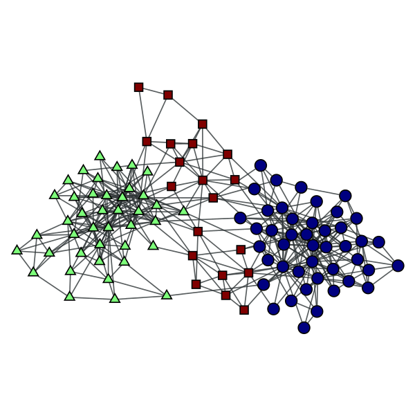
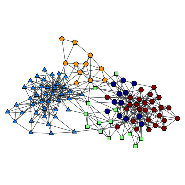
Block partition of a political books network, which minimizes the description lenght of the network according to the degree-corrected stochastic blockmodel.

class graph_tool.community.BlockState(g, eweight=None, vweight=None, b=None, clabel=None, B=None, deg_corr=True)

This class encapsulates the block state of a given graph.

This must be instantiated and used by functions such as mcmc_sweep().

Parameters :

g : Graph

Graph to be used.

eweight : PropertyMap (optional, default: None)

Edge weights (i.e. multiplicity).

vweight : PropertyMap (optional, default: None)

Vertex weights (i.e. multiplicity).

b : PropertyMap (optional, default: None)

Initial block labels on the vertices. If not supplied, it will be randomly sampled.

B : int (optional, default: None)

Number of blocks. If not supplied it will be either obtained from the parameter b, or set to the maximum possible value according to the minimum description length.

clabel : PropertyMap (optional, default: None)

This parameter provides a constraint label, such that vertices with different labels will not be allowed to belong to the same block. If not given, all labels will be assumed to be the same.

deg_corr : bool (optional, default: True)

If True, the degree-corrected version of the blockmodel ensemble will be assumed, otherwise the traditional variant will be used.

add_vertex(self, v, r)

Add vertex v to block r.

dist(self, r, s)

Compute the “distance” between blocks r and s, i.e. the entropy difference after they are merged together.

entropy(self, complete=False, random=False, dl=False)

Calculate the entropy per edge associated with the current block partition.

Parameters :

complete : bool (optional, default: False)

If True, the complete entropy will be returned, including constant terms not relevant to the block partition.

random : bool (optional, default: False)

If True, the entropy entropy corresponding to an equivalent random graph (i.e. no block partition) will be returned.

dl : bool (optional, default: False)

If True, the full description length will be returned.

Notes

For the traditional blockmodel (deg_corr == False), the entropy is given by

\[\begin{split}\mathcal{S}_t &\cong E - \frac{1}{2} \sum_{rs}e_{rs}\ln\left(\frac{e_{rs}}{n_rn_s}\right), \\ \mathcal{S}^d_t &\cong E - \sum_{rs}e_{rs}\ln\left(\frac{e_{rs}}{n_rn_s}\right),\end{split}\]

for undirected and directed graphs, respectively, where \(e_{rs}\) is the number of edges from block \(r\) to \(s\) (or the number of half-edges for the undirected case when \(r=s\)), and \(n_r\) is the number of vertices in block \(r\) .

For the degree-corrected variant with “hard” degree constraints the equivalent expressions are

\[\begin{split}\mathcal{S}_c &\cong -E -\sum_kN_k\ln k! - \frac{1}{2} \sum_{rs}e_{rs}\ln\left(\frac{e_{rs}}{e_re_s}\right), \\ \mathcal{S}^d_c &\cong -E -\sum_{k^+}N_{k^+}\ln k^+! -\sum_{k^-}N_{k^-}\ln k^-! - \sum_{rs}e_{rs}\ln\left(\frac{e_{rs}}{e^+_re^-_s}\right),\end{split}\]

where \(e_r = \sum_se_{rs}\) is the number of half-edges incident on block \(r\), and \(e^+_r = \sum_se_{rs}\) and \(e^-_r = \sum_se_{sr}\) are the number of out- and in-edges adjacent to block \(r\), respectively.

If complete == False only the last term of the equations above will be returned. If random == True it will be assumed that \(B=1\) despite the actual \(e_{rs}\) matrix. If dl == True, the description length \(\mathcal{L}_t\) of the model will be returned as well, as described in model_entropy(). Note that for the degree-corrected version the description length is

\[\mathcal{L}_c = \mathcal{L}_t - N\sum_kp_k\ln p_k,\]

where \(p_k\) is the fraction of nodes with degree \(p_k\), and we have instead \(k \to (k^-, k^+)\) for directed graphs.

Note that the value returned corresponds to the entropy per edge, i.e. \((\mathcal{S}_{t/c}\; [\,+\, \mathcal{L}_{t/c}])/ E\).

get_bg(self)

Returns the block graph.

get_blocks(self)

Returns the property map which contains the block labels for each vertex.

get_clabel(self)

Obtain the constraint label associated with each block.

get_dist_matrix(self)

Return the distance matrix between all blocks. The distance is defined as the entropy difference after two blocks are merged.

get_er(self)

Returns the vertex property map of the block graph which contains the number \(e_r\) of half-edges incident on block \(r\). If the graph is directed, a pair of property maps is returned, with the number of out-edges \(e^+_r\) and in-edges \(e^-_r\), respectively.

get_ers(self)

Returns the edge property map of the block graph which contains the \(e_{rs}\) matrix entries.

get_eweight(self)

Returns the block edge counts associated with the block matrix \(e_{rs}\). For directed graphs it is identical to \(e_{rs}\), but for undirected graphs it is identical except for the diagonal, which is \(e_{rr}/2\).

get_matrix(self, reorder=False, clabel=None, niter=0, ret_order=False)

Returns the block matrix.

Parameters :

reorder : bool (optional, default: False)

If True, the matrix is reordered so that blocks which are ‘similar’ are close together.

clabel : PropertyMap (optional, default: None)

Constraint labels to be imposed during reordering. Only has effect if reorder == True.

niter : int (optional, default: 0)

Number of iterations performed to obtain the best ordering. If niter == 0 it will automatically determined. Only has effect if reorder == True.

ret_order : bool (optional, default: False)

If True, the vertex ordering is returned. Only has effect if reorder == True.

Examples

>>> g = gt.collection.data["polbooks"]
>>> state = gt.BlockState(g, B=5, deg_corr=True)
>>> for i in range(1000):
...     ds, nmoves = gt.mcmc_sweep(state)
>>> m = state.get_matrix(reorder=True)
>>> figure()
<...>
>>> matshow(m)
<...>
>>> savefig("bloc_mat.pdf")

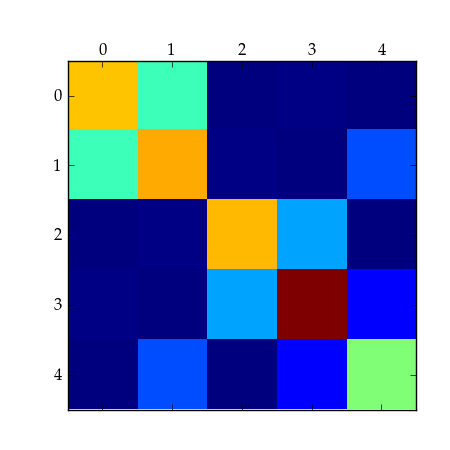
A 5x5 block matrix.

get_nr(self)

Returns the vertex property map of the block graph which contains the block sizes \(n_r\).

join(self, r, s)

Merge blocks r and s into a single block.

modularity(self)

Computes the modularity of the current block structure.

move_vertex(self, v, nr)

Move vertex v to block r, and return the entropy difference.

remove_vertex(self, v)

Remove vertex v from its current block.

graph_tool.community.mcmc_sweep(state, beta=1.0, sequential=True, verbose=False, vertices=None)

Performs a Monte Carlo Markov chain sweep on the network, to sample the block partition according to a probability \(\propto e^{-\beta \mathcal{S}_{t/c}}\), where \(\mathcal{S}_{t/c}\) is the blockmodel entropy.

Parameters :

state : BlockState

The block state.

beta : float (optional, default: 1.0)

The inverse temperature parameter \(\beta\).

sequential : bool (optional, default: True)

If True, the move attempts on the vertices are done in sequential random order. Otherwise a total of N moves attempts are made, where N is the number of vertices, where each vertex can be selected with equal probability.

verbose : bool (optional, default: False)

If True, verbose information is displayed.

Returns :

dS : float

The entropy difference (per edge) after a full sweep.

nmoves : int

The number of accepted block membership moves.

Notes

This algorithm performs a Monte Carlo Markov chain sweep on the network, where the block memberships are randomly moved, and either accepted or rejected, so that after sufficiently many sweeps the partitions are sampled with probability proportional to \(e^{-\beta\mathcal{S}_{t/c}}\), where \(\mathcal{S}_{t/c}\) is the blockmodel entropy, given by

\[\begin{split}\mathcal{S}_t &\cong - \frac{1}{2} \sum_{rs}e_{rs}\ln\left(\frac{e_{rs}}{n_rn_s}\right), \\ \mathcal{S}^d_t &\cong - \sum_{rs}e_{rs}\ln\left(\frac{e_{rs}}{n_rn_s}\right),\end{split}\]

for undirected and directed traditional blockmodels (deg_corr == False), respectively, where \(e_{rs}\) is the number of edges from block \(r\) to \(s\) (or the number of half-edges for the undirected case when \(r=s\)), and \(n_r\) is the number of vertices in block \(r\), and constant terms which are independent of the block partition were dropped (see BlockState.entropy() for the complete entropy). For the degree-corrected variant with “hard” degree constraints the equivalent expressions are

\[\begin{split}\mathcal{S}_c &\cong - \frac{1}{2} \sum_{rs}e_{rs}\ln\left(\frac{e_{rs}}{e_re_s}\right), \\ \mathcal{S}^d_c &\cong - \sum_{rs}e_{rs}\ln\left(\frac{e_{rs}}{e^+_re^-_s}\right),\end{split}\]

where \(e_r = \sum_se_{rs}\) is the number of half-edges incident on block \(r\), and \(e^+_r = \sum_se_{rs}\) and \(e^-_r = \sum_se_{sr}\) are the number of out- and in-edges adjacent to block \(r\), respectively.

The Monte Carlo algorithm employed attempts to improve the mixing time of the markov chain by proposing membership moves \(r\to s\) with probability \(p(r\to s|t) \propto e_{ts} + 1\), where \(t\) is the block label of a random neighbour of the vertex being moved. See [peixoto-parsimonious-2013] for more details.

This algorithm has a complexity of \(O(E)\), where \(E\) is the number of edges in the network.

References

[holland-stochastic-1983]

Paul W. Holland, Kathryn Blackmond Laskey, Samuel Leinhardt, “Stochastic blockmodels: First steps”, Carnegie-Mellon University, Pittsburgh, PA 15213, U.S.A., DOI: 10.1016/0378-8733(83)90021-7

[faust-blockmodels-1992]

Katherine Faust, and Stanley Wasserman. “Blockmodels: Interpretation and Evaluation.” Social Networks 14, no. 1-2 (1992): 5-61. DOI: 10.1016/0378-8733(92)90013-W

[karrer-stochastic-2011]

Brian Karrer, and M. E. J. Newman. “Stochastic Blockmodels and Community Structure in Networks.” Physical Review E 83, no. 1 (2011): 016107. DOI: 10.1103/PhysRevE.83.016107.

[peixoto-entropy-2012]

Tiago P. Peixoto “Entropy of Stochastic Blockmodel Ensembles.” Physical Review E 85, no. 5 (2012): 056122. DOI: 10.1103/PhysRevE.85.056122, arXiv: 1112.6028.

[peixoto-parsimonious-2013]

Tiago P. Peixoto, “Parsimonious module inference in large networks”, Phys. Rev. Lett. 110, 148701 (2013), DOI: 10.1103/PhysRevLett.110.148701, arXiv: 1212.4794.

Examples

>>> g = gt.collection.data["polbooks"]
>>> state = gt.BlockState(g, B=3, deg_corr=True)
>>> pv = None
>>> for i in range(1000):        # remove part of the transient
...     ds, nmoves = gt.mcmc_sweep(state)
>>> for i in range(1000):
...     ds, nmoves = gt.mcmc_sweep(state)
...     pv = gt.collect_vertex_marginals(state, pv)
>>> gt.graph_draw(g, pos=g.vp["pos"], vertex_shape="pie", vertex_pie_fractions=pv, output="polbooks_blocks_soft.pdf")
<...>

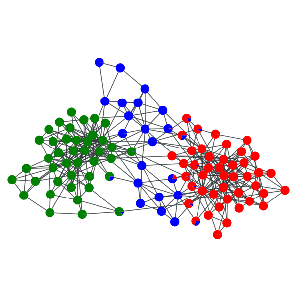
“Soft” block partition of a political books network with \(B=3\).

graph_tool.community.collect_edge_marginals(state, p=None)

Collect the edge marginal histogram, which counts the number of times the endpoints of each node have been assigned to a given block pair.

This should be called multiple times, after repeated runs of the mcmc_sweep() function.

Parameters :

state : BlockState

The block state.

p : PropertyMap (optional, default: None)

Edge property map with vector-type values, storing the previous block membership counts. Each vector entry corresponds to b[i] + B * b[j], where b is the block membership and i = min(source(e), target(e)) and j = max(source(e), target(e)). If not provided, an empty histogram will be created.

Returns :

p : PropertyMap (optional, default: None)

Vertex property map with vector-type values, storing the accumulated block membership counts.

Examples

>>> g = gt.collection.data["polbooks"]
>>> state = gt.BlockState(g, B=4, deg_corr=True)
>>> pe = None
>>> for i in range(1000):        # remove part of the transient
...     ds, nmoves = gt.mcmc_sweep(state)
>>> for i in range(1000):
...     ds, nmoves = gt.mcmc_sweep(state)
...     pe = gt.collect_edge_marginals(state, pe)
>>> gt.bethe_entropy(state, pe)[0]
17.17007316834295

graph_tool.community.collect_vertex_marginals(state, p=None)

Collect the vertex marginal histogram, which counts the number of times a node was assigned to a given block.

This should be called multiple times, after repeated runs of the mcmc_sweep() function.

Parameters :

state : BlockState

The block state.

p : PropertyMap (optional, default: None)

Vertex property map with vector-type values, storing the previous block membership counts. If not provided, an empty histogram will be created.

Returns :

p : PropertyMap (optional, default: None)

Vertex property map with vector-type values, storing the accumulated block membership counts.

Examples

>>> g = gt.collection.data["polbooks"]
>>> state = gt.BlockState(g, B=4, deg_corr=True)
>>> pv = None
>>> for i in range(1000):        # remove part of the transient
...     ds, nmoves = gt.mcmc_sweep(state)
>>> for i in range(1000):
...     ds, nmoves = gt.mcmc_sweep(state)
...     pv = gt.collect_vertex_marginals(state, pv)
>>> gt.mf_entropy(state, pv)
20.001666525168361
>>> gt.graph_draw(g, pos=g.vp["pos"], vertex_shape="pie", vertex_pie_fractions=pv, output="polbooks_blocks_soft_B4.pdf")
<...>

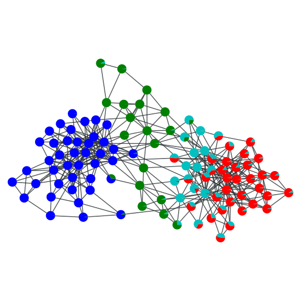
“Soft” block partition of a political books network with \(B=4\).

graph_tool.community.bethe_entropy(state, p)

Compute the Bethe entropy given the edge block membership marginals.

Parameters :

state : BlockState

The block state.

p : PropertyMap

Edge property map with vector-type values, storing the previous block membership counts. Each vector entry corresponds to b[i] + B * b[j], where b is the block membership and i = min(source(e), target(e)) and j = max(source(e), target(e)).

Returns :

H : float

The Bethe entropy value (in nats)

Hmf : float

The “mean field” entropy value (in nats), as would be returned by the mf_entropy() function.

pv : PropertyMap (optional, default: None)

Vertex property map with vector-type values, storing the accumulated block membership counts. These are the node marginals, as would be returned by the collect_vertex_marginals() function.

Notes

The Bethe entropy is defined as,

\[H = -\sum_{e,(r,s)}\pi_{(r,s)}^e\ln\pi_{(r,s)}^e - \sum_{v,r}(1-k_i)\pi_r^v\ln\pi_r^v,\]

where \(\pi_{(r,s)}^e\) is the marginal probability that the endpoints of the edge \(e\) belong to blocks \((r,s)\), and \(\pi_r^v\) is the marginal probability that vertex \(v\) belongs to block \(r\), and \(k_i\) is the degree of vertex \(v\) (or total degree for directed graphs).

References

[mezard-information-2009]

Marc Mézard, Andrea Montanari, “Information, Physics, and Computation”, Oxford Univ Press, 2009.

graph_tool.community.mf_entropy(state, p)

Compute the “mean field” entropy given the vertex block membership marginals.

Parameters :

state : BlockState

The block state.

p : PropertyMap

Vertex property map with vector-type values, storing the accumulated block membership counts.

Returns :

Hmf : float

The “mean field” entropy value (in nats).

Notes

The “mean field” entropy is defined as,

\[H = - \sum_{v,r}\pi_r^v\ln\pi_r^v,\]

where \(\pi_r^v\) is the marginal probability that vertex \(v\) belongs to block \(r\).

References

[mezard-information-2009]

Marc Mézard, Andrea Montanari, “Information, Physics, and Computation”, Oxford Univ Press, 2009.

graph_tool.community.model_entropy(B, N, E, directed)

Computes the amount of information necessary for the parameters of the traditional blockmodel ensemble, for B blocks, N vertices, E edges, and either a directed or undirected graph.

A traditional blockmodel is defined as a set of \(N\) vertices which can belong to one of \(B\) blocks, and the matrix \(e_{rs}\) describes the number of edges from block \(r\) to \(s\) (or twice that number if \(r=s\) and the graph is undirected).

For an undirected graph, the number of distinct \(e_{rs}\) matrices is given by,

\[\Omega_m = \left(\!\!{\left(\!{B \choose 2}\!\right) \choose E}\!\!\right)\]

and for a directed graph,

\[\Omega_m = \left(\!\!{B^2 \choose E}\!\!\right)\]

where \(\left(\!{n \choose k}\!\right) = {n+k-1\choose k}\) is the number of \(k\) combinations with repetitions from a set of size \(n\).

The total information necessary to describe the model is then,

\[\mathcal{L}_t = \ln\Omega_m + N\ln B,\]

where \(N\ln B\) is the information necessary to describe the block partition.

References

[peixoto-parsimonious-2013]

Tiago P. Peixoto, “Parsimonious module inference in large networks”, Phys. Rev. Lett. 110, 148701 (2013), DOI: 10.1103/PhysRevLett.110.148701, arXiv: 1212.4794.

graph_tool.community.get_max_B(N, E, directed=False)

Return the maximum detectable number of blocks, obtained by minimizing:

\[\mathcal{L}_t(B, N, E) - E\ln B\]

where \(\mathcal{L}_t(B, N, E)\) is the information necessary to describe a traditional blockmodel with B blocks, N nodes and E edges (see model_entropy()).

References

[peixoto-parsimonious-2013]

Tiago P. Peixoto, “Parsimonious module inference in large networks”, Phys. Rev. Lett. 110, 148701 (2013), DOI: 10.1103/PhysRevLett.110.148701, arXiv: 1212.4794.

Examples

>>> gt.get_max_B(N=1e6, E=5e6)
1572

graph_tool.community.get_akc(B, I, N=inf, directed=False)

Return the minimum value of the average degree of the network, so that some block structure with \(B\) blocks can be detected, according to the minimum description length criterion.

This is obtained by solving

\[\Sigma_b = \mathcal{L}_t(B, N, E) - E\mathcal{I}_{t/c} = 0,\]

where \(\mathcal{L}_{t}\) is the necessary information to describe the blockmodel parameters (see model_entropy()), and \(\mathcal{I}_{t/c}\) characterizes the planted block structure, and is given by

\[\begin{split}\mathcal{I}_t &= \sum_{rs}m_{rs}\ln\left(\frac{m_{rs}}{w_rw_s}\right),\\ \mathcal{I}_c &= \sum_{rs}m_{rs}\ln\left(\frac{m_{rs}}{m_rm_s}\right),\end{split}\]

where \(m_{rs} = e_{rs}/2E\) (or \(m_{rs} = e_{rs}/E\) for directed graphs) and \(w_r=n_r/N\). We note that \(\mathcal{I}_{t/c}\in[0, \ln B]\). In the case where \(E \gg B^2\), this simplifies to

\[\begin{split}\left<k\right>_c &= \frac{2\ln B}{\mathcal{I}_{t/c}},\\ \left<k^{-/+}\right>_c &= \frac{\ln B}{\mathcal{I}_{t/c}},\end{split}\]

for undirected and directed graphs, respectively. This limit is assumed if N == inf.

References

[peixoto-parsimonious-2013]

Tiago P. Peixoto, “Parsimonious module inference in large networks”, Phys. Rev. Lett. 110, 148701 (2013), DOI: 10.1103/PhysRevLett.110.148701, arXiv: 1212.4794.

Examples

>>> gt.get_akc(10, log(10) / 100, N=100)
2.4199998936261204

graph_tool.community.min_dist(state, n=0)

Return the minimum distance between all blocks, and the block pair which minimizes it.

The parameter state must be an instance of the BlockState class, and n is the number of block pairs to sample. If n == 0 all block pairs are sampled.

Examples

>>> g = gt.collection.data["polbooks"]
>>> state = gt.BlockState(g, B=4, deg_corr=True)
>>> for i in range(1000):
...     ds, nmoves = gt.mcmc_sweep(state)
>>> gt.min_dist(state)
(795.7694502418633, 2, 3)

graph_tool.community.condensation_graph(g, prop, vweight=None, eweight=None, avprops=None, aeprops=None, self_loops=False)

Obtain the condensation graph, where each vertex with the same ‘prop’ value is condensed in one vertex.

Parameters :

g : Graph

Graph to be used.

prop : PropertyMap

Vertex property map with the community partition.

vweight : PropertyMap (optional, default: None)

Vertex property map with the optional vertex weights.

eweight : PropertyMap (optional, default: None)

Edge property map with the optional edge weights.

avprops : list of PropertyMap (optional, default: None)

If provided, the average value of each property map in this list for each vertex in the condensed graph will be computed and returned.

aeprops : list of PropertyMap (optional, default: None)

If provided, the average value of each property map in this list for each edge in the condensed graph will be computed and returned.

self_loops : bool (optional, default: False)

If True, self-loops due to intra-block edges are also included in the condensation graph.

Returns :

condensation_graph : Graph

The community network

prop : PropertyMap

The community values.

vcount : PropertyMap

A vertex property map with the vertex count for each community.

ecount : PropertyMap

An edge property map with the inter-community edge count for each edge.

va : list of PropertyMap

A list of vertex property maps with average values of the properties passed via the avprops parameter.

ea : list of PropertyMap

A list of edge property maps with average values of the properties passed via the avprops parameter.

See also

community_structure

Obtain the community structure

modularity

Calculate the network modularity

condensation_graph

Network of communities, or blocks

Notes

Each vertex in the condensation graph represents one community in the original graph (vertices with the same ‘prop’ value), and the edges represent existent edges between vertices of the respective communities in the original graph.

Examples

Let’s first obtain the best block partition with B=5.

>>> g = gt.collection.data["polbooks"]
>>> state = gt.BlockState(g, B=5, deg_corr=True)
>>> for i in range(1000):        # remove part of the transient
...     ds, nmoves = gt.mcmc_sweep(state)
>>> for i in range(1000):
...     ds, nmoves = gt.mcmc_sweep(state, beta=float("inf"))
>>> b = state.get_blocks()
>>> gt.graph_draw(g, pos=g.vp["pos"], vertex_fill_color=b, vertex_shape=b, output="polbooks_blocks_B5.pdf")
<...>

Now we get the condensation graph:

>>> bg, bb, vcount, ecount, avp, aep = gt.condensation_graph(g, b, avprops=[g.vp["pos"]], self_loops=True)
>>> gt.graph_draw(bg, pos=avp[0], vertex_fill_color=bb, vertex_shape=bb,
...               vertex_size=gt.prop_to_size(vcount, mi=40, ma=100),
...               edge_pen_width=gt.prop_to_size(ecount, mi=2, ma=10),
...               output="polbooks_blocks_B5_cond.pdf")
<...>

Block partition of a political books network with \(B=5\).

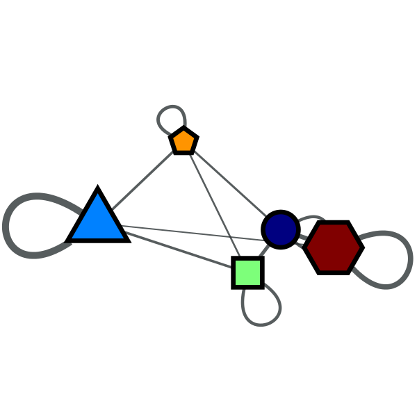
Condensation graph of the obtained block partition.

graph_tool.community.community_structure(g, n_iter, n_spins, gamma=1.0, corr='erdos', spins=None, weight=None, t_range=(100.0, 0.01), verbose=False, history_file=None)

Obtain the community structure for the given graph, using a Potts model approach.

Parameters :

g : Graph

Graph to be used.

n_iter : int

Number of iterations.

n_spins : int

Number of maximum spins to be used.

gamma : float (optional, default: 1.0)

The \(\gamma\) parameter of the hamiltonian.

corr : string (optional, default: “erdos”)

Type of correlation to be assumed: Either “erdos”, “uncorrelated” and “correlated”.

spins : PropertyMap

Vertex property maps to store the spin variables. If this is specified, the values will not be initialized to a random value.

weight : PropertyMap (optional, default: None)

Edge property map with the optional edge weights.

t_range : tuple of floats (optional, default: (100.0, 0.01))

Temperature range.

verbose : bool (optional, default: False)

Display verbose information.

history_file : string (optional, default: None)

History file to keep information about the simulated annealing.

Returns :

spins : PropertyMap

Vertex property map with the spin values.

See also

community_structure

Obtain the community structure

modularity

Calculate the network modularity

condensation_graph

Network of communities, or blocks

Notes

The method of community detection covered here is an implementation of what was proposed in [reichard-statistical-2006]. It consists of a simulated annealing algorithm which tries to minimize the following hamiltonian:

\[\mathcal{H}(\{\sigma\}) = - \sum_{i \neq j} \left(A_{ij} - \gamma p_{ij}\right) \delta(\sigma_i,\sigma_j)\]

where \(p_{ij}\) is the probability of vertices i and j being connected, which reduces the problem of community detection to finding the ground states of a Potts spin-glass model. It can be shown that minimizing this hamiltonan, with \(\gamma=1\), is equivalent to maximizing Newman’s modularity ([newman-modularity-2006]). By increasing the parameter \(\gamma\), it’s possible also to find sub-communities.

It is possible to select three policies for choosing \(p_{ij}\) and thus choosing the null model: “erdos” selects a Erdos-Reyni random graph, “uncorrelated” selects an arbitrary random graph with no vertex-vertex correlations, and “correlated” selects a random graph with average correlation taken from the graph itself. Optionally a weight property can be given by the weight option.

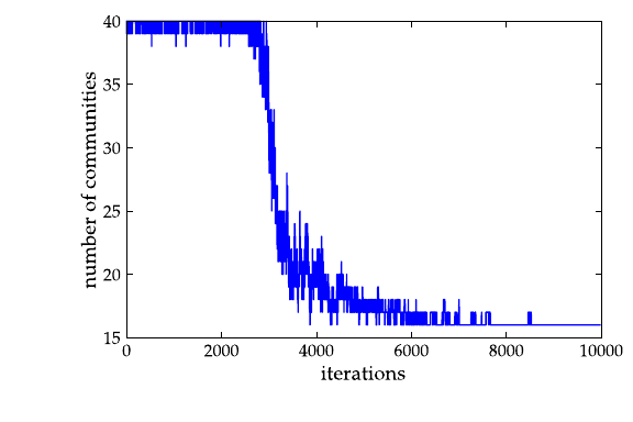
The most important parameters for the algorithm are the initial and final temperatures (t_range), and total number of iterations (max_iter). It normally takes some trial and error to determine the best values for a specific graph. To help with this, the history option can be used, which saves to a chosen file the temperature and number of spins per iteration, which can be used to determined whether or not the algorithm converged to the optimal solution. Also, the verbose option prints the computation status on the terminal.

Note

If the spin property already exists before the computation starts, it’s not re-sampled at the beginning. This means that it’s possible to continue a previous run, if you saved the graph, by properly setting t_range value, and using the same spin property.

If enabled during compilation, this algorithm runs in parallel.

References

[reichard-statistical-2006]

(1, 2) Joerg Reichardt and Stefan Bornholdt, “Statistical Mechanics of Community Detection”, Phys. Rev. E 74 016110 (2006), DOI: 10.1103/PhysRevE.74.016110, arXiv: cond-mat/0603718

[newman-modularity-2006]

M. E. J. Newman, “Modularity and community structure in networks”, Proc. Natl. Acad. Sci. USA 103, 8577-8582 (2006), DOI: 10.1073/pnas.0601602103, arXiv: physics/0602124

Examples

This example uses the network community.xml.

>>> from pylab import *
>>> from numpy.random import seed
>>> seed(42)
>>> g = gt.load_graph("community.xml")
>>> pos = g.vertex_properties["pos"]
>>> spins = gt.community_structure(g, 10000, 20, t_range=(5, 0.1),
...                                history_file="community-history1")
>>> gt.graph_draw(g, pos=pos, vertex_fill_color=spins, output_size=(420, 420), output="comm1.pdf")
<...>
>>> spins = gt.community_structure(g, 10000, 40, t_range=(5, 0.1),
...                                gamma=2.5, history_file="community-history2")
>>> gt.graph_draw(g, pos=pos, vertex_fill_color=spins, output_size=(420, 420), output="comm2.pdf")
<...>
>>> figure(figsize=(6, 4))
<...>
>>> xlabel("iterations")
<...>
>>> ylabel("number of communities")
<...>
>>> a = loadtxt("community-history1").transpose()
>>> plot(a[0], a[2])
[...]
>>> savefig("comm1-hist.pdf")
>>> clf()
>>> xlabel("iterations")
<...>
>>> ylabel("number of communities")
<...>
>>> a = loadtxt("community-history2").transpose()
>>> plot(a[0], a[2])
[...]
>>> savefig("comm2-hist.pdf")

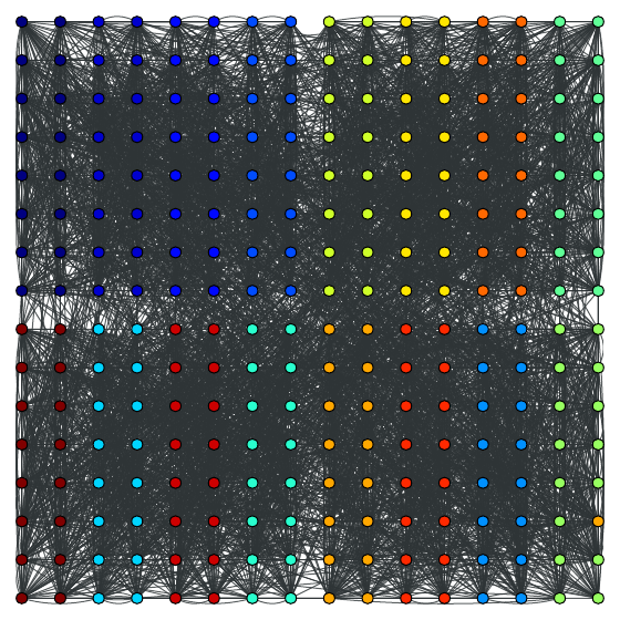
The community structure with \(\gamma=1\):

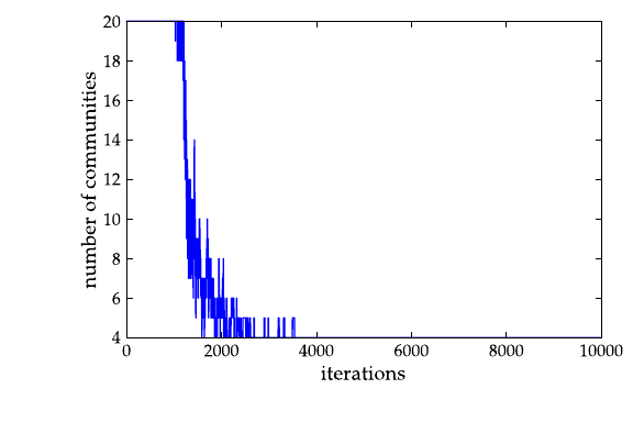
The community structure with \(\gamma=2.5\):

graph_tool.community.modularity(g, prop, weight=None)

Calculate Newman’s modularity.

Parameters :

g : Graph

Graph to be used.

prop : PropertyMap

Vertex property map with the community partition.

weight : PropertyMap (optional, default: None)

Edge property map with the optional edge weights.

Returns :

modularity : float

Newman’s modularity.

See also

community_structure

obtain the community structure

modularity

calculate the network modularity

condensation_graph

Network of communities, or blocks

Notes

Given a specific graph partition specified by prop, Newman’s modularity [newman-modularity-2006] is defined by:

\[Q = \sum_s e_{ss}-\left(\sum_r e_{rs}\right)^2\]

where \(e_{rs}\) is the fraction of edges which fall between vertices with spin s and r.

If enabled during compilation, this algorithm runs in parallel.

References

[newman-modularity-2006]

M. E. J. Newman, “Modularity and community structure in networks”, Proc. Natl. Acad. Sci. USA 103, 8577-8582 (2006), DOI: 10.1073/pnas.0601602103, arXiv: physics/0602124

Examples

>>> from pylab import *
>>> from numpy.random import seed
>>> seed(42)
>>> g = gt.load_graph("community.xml")
>>> spins = gt.community_structure(g, 10000, 10)
>>> gt.modularity(g, spins)
0.535314188562404